
- Pros (+): Theoretical justification, simple model, easy to implement.
- Cons (-): Some training instability in practice.
Generalized Bound on the Expected Risk
Several theoretical studies of the domain adaptation problem have proposed upper bounds of the risk on the target domain, involving the risk on the source domain and a notion of distance between the source and target distribution, \(\mathcal D_S\) and \(\mathcal D_T\). Here, the authors specifically consider the work of [1]. First, they define the \(\mathcal H\)-divergence:
\[\begin{align} d_{\mathcal H}(\mathcal D_S, \mathcal D_T) = 2 \sup_{h \in \mathcal H} \left| \mathbb{E}_{x\sim\mathcal{D}_s} (h(x) = 1) - \mathbb{E}_{x\sim\mathcal{D}_T} (h(x) = 1) \right| \tag{1} \end{align}\]where \(\mathcal H\) is a space of (here, binary) hypothesis functions. In the case where \(\mathcal H\) is a symmetric hypothesis class (i.e., \(h \in \mathcal H \implies -h \in \mathcal H\)), one can reduce (1) to the empirical form:
\[\begin{align} d_{\mathcal H}(\mathcal D_S, \mathcal D_T) &\simeq 2 \sup_{h \in \mathcal H} \left|\frac{1}{|D_S|} \sum_{x \in D_S} [\!|h(x) = 1 |\!] - \frac{1}{|D_T|} \sum_{x \in D_T} [\!|h(x) = 1 |\!] \right|\\ &= 2 \sup_{h \in \mathcal H} \left|\frac{1}{|D_S|} \sum_{x \in D_S} 1 - [\!|h(x) = 0 |\!] - \frac{1}{|D_T|} \sum_{x \in D_T} [\!|h(x) = 1 |\!] \right|\\ &= 2 - 2 \min_{h \in \mathcal H} \left|\frac{1}{|D_S|} \sum_{x \in D_S} [\!|h(x) = 0 |\!] + \frac{1}{|D_T|} \sum_{x \in D_T} [\!|h(x) = 1 |\!] \right| \tag{2} \end{align}\]It is difficult to estimate the minimum over the hypothesis class \(\mathcal H\). Instead, [1] propose to approximate Equation (2) by training a classifier \(\hat{h}\) on samples \(\mathbf{x_S} \in \mathcal{D}_S\) with label 0 and \(\mathbf{x_T} \in \mathcal D_T\) with label 1, and replacing the minimum term by the empirical risk of \(\hat h\). Given this definition of the \(\mathcal H\)-divergence, [1] further derives an upper bound on the empirical risk on the target domain, which in particular involves a trade-off between the empirical risk on the source domain, \(\mathcal{R}_{D_S}(h)\), and the divergence between the source and target distributions, \(d_{\mathcal H}(D_S, D_T)\).
where \(\mbox{VC}\) designates the Vapnik–Chervonenkis dimensions and \(n\) the number of samples. The rest of the paper directly stems from this intuition: in order to minimize the target risk the proposed Domain Adversarial Neural Network (DANN) aims to build an “internal representation that contains no discriminative information about the origin of the input (source or target), while preserving a low risk on the source (labeled) examples”.
Proposed
The goal of the model is to learn a classifier \(\phi\), which can be decomposed as \(\phi = G_y \circ G_f\), where \(G_f\) is a feature extractor and \(G_y\) a small classifier on top that outputs the target label. This architecture is trained with a standard classification objective to minimize:
\[\begin{align} \mathcal{L}_y(\theta_f, \theta_y) = \frac{1}{N_s} \sum_{(x, y) \in D_s} \ell(G_y(G_f(x)), y) \end{align}\]Additionally DANN introduces a domain prediction branch, which is another classifier \(G_d\) on top of the feature representation \(G_f\) and whose goal is to approximate the domain discrepancy as (2), which leads to the following training objective to maximize:
The final objective can thus be written as:
\[\begin{align} E(\theta_f, \theta_y, \theta_d) &= \mathcal{L}_y(\theta_f, \theta_y) - \lambda \mathcal{L}_d(\theta_f, \theta_d) \tag{1}\\ \theta_f^\ast, \theta_y^\ast &= \arg\min E(\theta_f, \theta_y, \theta_d) \tag{2}\\ \theta_d^\ast &= \arg\max E(\theta_f, \theta_y, \theta_d) \tag{3} \end{align}\]Gradient Reversal Layer
Applying standard gradient descent, the DANN objective leads to the following gradient update rules:
In the case of neural networks, the gradients of the loss with respect to parameters are obtained with the backpropagation algorithm. The current system equations are very similar to the standard backpropagation scheme, except for the opposite sign in the derivative of \(\mathcal{L}_d\) with respect to \(\theta_d\) and \(\theta_f\). The authors introduce the gradient reversal layer (GRL) to evaluate both gradients in one standard backpropagation step.
The idea is that the output of \(\theta_f\) is normally propagated to \(\theta_d\), however during backpropagation, its gradient is multiplied by a negative constant:
\[\begin{align} \frac{\partial \mathcal L_d}{\partial \theta_f} = \frac{\bf{\color{red}{-}} \partial \mathcal L_d}{\partial G_f(x)} \frac{\partial G_f(x)}{\partial \theta_f} \end{align}\]In other words, for the update of \(\theta_d\), the gradients of \(\mathcal L_d\) with the respect to activations are computed normally (minimization), but they are then propagated with a minus sign in the feature extraction part of the network (maximization). Augmented with the gradient reversal layer, the final model is trained by minimizing the sum of losses \(\mathcal L_d + \mathcal L_y\) , which corresponds to the optimization problem in (1-3).
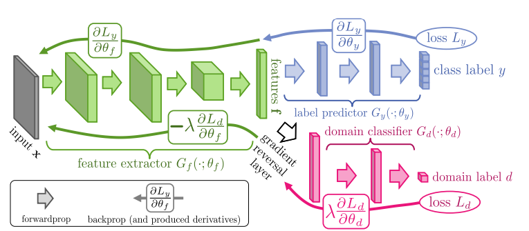
Figure: The proposed architecture includes a deep feature extractor and a deep label predictor. Unsupervised domain adaptation is achieved by adding a domain classifier connected to the feature extractor via a gradient reversal layer that multiplies the gradient by a certain negative constant during backpropagation.
Experiments
Datasets
The paper presents extensive results on the following settings:
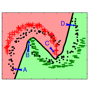
- Toy dataset: A toy example based on the two half-moons dataset, where the source domains consists in the standard binary classification tasks with the two half-moons, and the target is the same, but with a 30 degrees rotation. They compare the
DANNto aNNmodel which has the same architecture but without theGRL: in other words, the baseline directly minimizes both the task and domain classification losses. - Sentiment Analysis: These experiments are performed on the Amazon reviews dataset which contains product reviews from four different domains (hence 12 different source to target scenarios) which have to be classified as either positive or negative reviews.
- Image Classification: Here the model is evaluated on various image classification task including MNIST \(\rightarrow\) SVHN, or different domain pairs from the OFFICE dataset [2] .
- Person Re-identification: The task of person identification across various visual domains.
Validation
Setting hyperparameters is a difficult problem, as we cannot directly evaluate the model on the target domain (no labeled data available). Instead of standard cross-validation, the authors use reverse validation based on a technique introduced in [3]: First, the (labeled) source set \(S\) and (unlabeled) target set \(T\) are each split into a training and validation set, \(S'\) and \(S_V\) (resp. \(T'\) and \(T_V\)). Using these splits, a model \(\eta\) is trained on \(S'\rightarrow T'\). Then a second model \(\eta_r\) is trained for the reverse direction on the set \(\{ (x, \eta(x)),\ x \in T'\} \rightarrow S'\). This reverse classifier \(\eta_r\) is then finally evaluated on the labeled validation set \(S_V\), and this accuracy is used as a validation score.
Conclusions
In general, the proposed method seems to perform very well for aligning the source and target domains in an unsupervised domain adaptation framework. Its main advantage is its simplicity, both in terms of theoretical motivation and implementation. In fact, the GRL is easily implemented in standard Deep Learning frameworks and can be added to any architectures.
The main shortcomings of the method are that (i) all experiments deal with only two sources and extensions to multiple domains might require some tweaks (e.g., considering the sum of pairwise discrepancies as an upper-bound) and (ii) in practice, training can become unstable due to the adversary training scheme; In particular, the experiment sections show that some stability tricks have to be used during training, such as using momentum or slowly increasing the contribution of the domain classification branch.
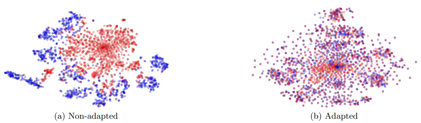
Figure: t-SNE projections of the embeddings for the source (MNIST) and target (SVHN) datasets without (left) and with (right) DANN adaptation.
Closely related
Conditional Adversarial Domain Adaptation.
Long et al, NeurIPS 2018[link]
In this work, the authors propose to for Domain Adversarial Networks. More specifically, the domain classifier is conditioned on the input’s class: However, since part of the samples are unlabeled, the conditioning uses the output of the target classifier branch as a proxy for the class information. Instead of simply concatenating the feature input with the condition, the authors consider a multilinear conditioning technique which relies on the cross-covariance operator. Another related paper is [4]. It also uses the multi-class information of the input domain, although in a simpler way.
References
- [1] Analysis of representations for Domain Adaptation, Ben-David et al, NeurIPS 2006
- [2] Adapting visual category models to new domains, Saenko et al, ECCV 2010
- [3] Person re-identification via structured prediction, Zhang and Saligrama, arXiv 2014
- [4] Multi-Adversarial Domain Adaptation, Pei et al, AAAI 2018