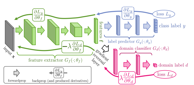
VQ-VAE, a variant of the Variational Autoencoder (VAE) framework with a discrete latent space, using ideas from vector quantization. The two main motivations are (i) discrete variables are potentially better fit to capture the structure of data such as text and (ii) to prevent the posterior collapse in VAEs that leads to latent variables being ignored when the decoder is too powerful.
- Pros (+): Simple method to incorporate a discretized latent space in VAEs.
- Cons (-): Paragraph about the learned prior is not very clear, and does not have corresponding ablation experiments to evalute its importance.
Proposed
Discrete latent space
The model is based on VAE [1], where image \(x\) is generated from random latent variable \(z\) by a decoder \(p(x\ \vert\ z)\). The posterior (encoder) captures the latent variable distribution \(q_{\phi}(z\ \vert\ x)\) and is generally trained to match a certain distribution \(p(z)\) from which \(z\) is sampled from at inference time.
Contrary to the standard framework, in this work the latent space is discrete, i.e., \(z \in \mathbb{R}^{K \times D}\) where \(K\) is the number of codes in the latent space and \(D\) their dimensionality. More precisely, the input image is first fed to \(z_e\), that outputs a continuous vector, which is then mapped to one of the latent codes in the discrete space via nearest-neighbor search.
Adapting the \(\mathcal{L}_{\text{ELBO}}\) to this formalism, the KL divergence term greatly simplifies and we obtain:
\[\begin{align} \mathcal{L}_{\text{ELBO}}(x) &= \text{KL}(q(z | x) \| p(z)) - \mathbb{E}_{z \sim q(\cdot | x)}(\log p(x | z))\\ &= - \log(p(z_k)) - \log p(x | z_k)\\ \mbox{where }& z_k = z_q(x) = \arg\min_z \| z_e(x) - z \|^2 \tag{1} \end{align}\]In practice, the authors use a categorical uniform prior for the latent codes, meaning the KL divergence is constant and the objective reduces to the reconstruction loss.
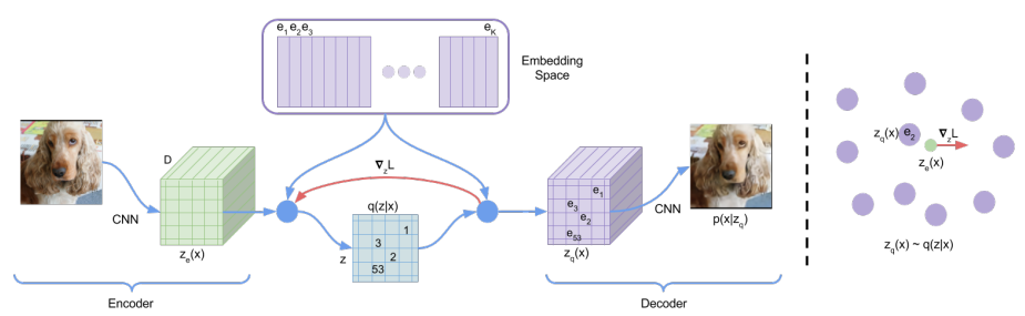
Figure: A figure describing the VQ-VAE (left). Visualization of the embedding space (right)). The output of the encoder z(x) is mapped to the nearest point. The gradient (in red) will push the
encoder to change its output, which could alter the configuration, hence the code assignment, in the next forward pass.
Training Objective
As we mentioned previously, the \(\mathcal{L}_{\text{ELBO}}\) objective reduces to the reconstruction loss and is used to learn the encoder and decoder parameters. However the mapping from \(z_e\) to \(z_q\) is not straight-forward differentiable (Equation (1)). To palliate this, the authors use a straight-through estimator, meaning the gradients from the decoder input \(z_q(x)\) (quantized) are directly copied to the encoder output \(z_e(x)\) (continuous). However, this means that the latent codes that intervene in the mapping from \(z_e\) to \(z_q\) do not receive gradient updates that way.
Hence in order to train the discrete embedding space, the authors propose to use Vector Quantization (VQ), a dictionary learning technique, which uses mean squared error to make the latent code closer to the continuous vector it was matched to:
where \(x \mapsto \overline{x}\) denotes the stop gradient operator. The first term is the reconstruction loss stemming from the ELBO, the second term is the vector quantization contribution. Finally, the last term is a commitment loss to control the volume of the latent space by forcing the encoder to “commit” to the latent code it matched with, and not grow its output space unbounded.
Learned Prior
A second contribution of this work consists in learning the prior distribution. As mentioned, during the training phase, the prior \(p(z)\) is a uniform categorical distribution. After the training is done, we fit an autoregressive distribution over the space of latent codes. This is in particular enabled by the fact that the latent space is discrete.
Note: It is not clear to me if the autoregressive model is trained on latent codes sampled from the prior \(z \sim p(z)\) or from the encoder distribution \(x \sim \mathcal{D};\ z \sim q(z\ \vert\ x)\)
Experiments
The proposed model is mostly compared to the standard continuous VAE framework. It seems to achieve similar log-likelihood and sample quality, while taking advantage of the discrete latent space. In particular
For ImageNet for instance, they consider \(K = 512\) latent codes with dimensions \(1\). The output of the fully-convolutional encoder \(z_e\) is a feature map of size \(32 \times 32 \times 1\) which is then quantized pixel-wise. Interestingly, the model still performs well when using a powerful decoder (here, PixelCNN [2]) which seems to indicate it does not suffer from posterior collapse as strongly as the standard continuous VAE.
A second set of experiments tackles the problem of audio modeling. The performance of the model are once again satisfying. Furthermore, it does seem like the discrete latent space actually captures relevant characteristics of the input data structure, although this is a purely qualitative observation.
References
- [1] Autoencoding Variational Bayes, Kingma and Welling, ICLR 2014
- [2] Pixel Recurrent Neural Networks, van den Oord et al, arXiv 2016