This post presents a short introduction and Tensorflow v1 (graph-based) implementation of the Variational Auto-encoder model (VAE) introduced in Auto-Encoding Variational Bayes, D. Kingma, M. Welling, ICLR 2017, with experiments on the CelebA faces dataset.
Model
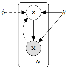
Variational Auto-encoders (VAE) are probabilistic generative models relying on a simple latent representation that captures the input data intrinsic properties. Given latent code \(z\) sampled from a prior distribution \(p_{\theta}(z)\), we generate a sample \(x\) from the conditional \(p_{\theta}(x\ |\ z)\). The goal is to learn the parameters of this generative model as well as how to map data points to latent codes.
In many cases however, the posterior distribution \(p_{\theta}(z\ |\ x)\) is intractable. It is instead approximated by a parametric model \(q_{\phi}(z\ |\ x)\), where \(\phi\) are called the variational parameters (see the graphical model below). In the following, we will drop the \(\theta\) and \(\phi\) notations for simplicity.

To summarize, a VAE is composed from an encoder \(q(z\ |\ x)\), which maps an input \(x\) to a latent representation \(z\), typically of much lower dimension, and a decoder \(p(x\ |\ z)\) that generates sample \(x\) from a latent code \(z\). Both of these mappings are parametrized as neural networks in practice, and our goal is to find their optimal parameters by maximizing the data likelihood, \(p(x)\).
Training objective
As the likelihood is intractable, we indeed derive the following variational lower bound (also known as \({\mathcal L}_{ELBO}\)) on the data log-likelihood:
The model is trained by minimizing \({\mathcal L}_{ELBO}\); The right term is typically interpreted as a reconstruction loss term, given codes sampled from the encoder distribution, while the left term acts as a regularizer and is the KL divergence between the approximate posterior and the prior \(p(z)\). Finally, note that this bound is optimal when the encoder perfectly approximates the true posterior, i.e., \(\mbox{KL}(q(z\ |\ x)\ \|\ p(z\ |\ x)) = 0\).
Parametrization
The vanilla VAE is parametrized with Gaussian function as follows:
- The latent code prior is \(p(z) = \mathcal{N}(z\ |\ 0, 1)\)
- \(q(z\ |\ x) = \mathcal{N}(z\ |\ \mu_q(x), \sigma_q(x))\) is a Gaussian with diagonal covariance, where \(\mu_q\) and \(\sigma_q\) are output by the encoder network.
- \(p(x\ |\ z) = \mathcal{N}(x\ |\ \mu_p(z), \sigma_p)\) is a Gaussian with diagonal covariance, where \(\mu_p\) is the reconstruction output by the decoder network and \(\sigma_p \in \mathbb{R}\) is an hyperparameter.
Implementation
Inputs pipeline
First, we define the input loading queue which reads images from a given list of filenames and feeds them through an optional preprocessing function. I use Tensorflow queues utilities rather than placeholder so all input-related operations are built in the static graph directly.
The get_inputs_queue function returns a queue whose elements are input dictionary with key “image”: A 4D Tensor of size (batch_size, height, width, num_channels) representing the inputs.
# Read Image from file
inputs = {}
filename_queue = tf.train.string_input_producer(
    filenames, capacity=capacity, shuffle=False)
_, reader = tf.WholeFileReader().read(filename_queue)
image = tf.image.decode_jpeg(reader, channels=channels, name='decoder')
inputs['image'] = image

# Preprocess the inputs
with tf.variable_scope('inputs_preprocess'):
    inputs = preprocess_inputs(inputs)

# Batch and shuffle the inputs
inputs = tf.train.shuffle_batch(
    inputs,  batch_size, capacity, min_after_dequeue)
The preprocess_inputs function simply performs a central crop on the input image, resizes them to square size 128x128 and finally maps them to [-1, 1].
# Map to [-1, 1]
with tf.control_dependencies([tf.assert_type(inputs['image'], tf.uint8)]):
   inputs['image'] = tf.image.convert_image_dtype(
       inputs['image'], tf.float32)
   inputs['image'] = (inputs['image'] - 0.5) * 2

# Central crop to minimal side
height = tf.shape(inputs['image'])[0]
width = tf.shape(inputs['image'])[1]
min_side =  tf.minimum(height, width)
offset_height = (height - min_side) // 2
offset_width = (width - min_side) // 2
inputs['image'] = tf.image.crop_to_bounding_box(
    inputs['image'], offset_height, offset_width, min_side, min_side)

# Resize
if size is not None and size > 0:
    inputs['image'] = tf.image.resize_images(inputs['image'], (size, size))
Architecture
For the feed-forward network, I use a rather simple convolutional architecture with ReLU activations, batch normalization layers and max-pooling. More specifically, the encoder is described and implemented as follow
Encoder
- Inputs: (batch size, 128, 128, 3) in [-1, 1]
- 5 convolutional blocks
- Convolutions, stride 2
- ReLU activation and Batch normalization
- Max-pooling
- Final block: (batch size, 4, 4, c)
- 2 separate fully-connected layers
- Outputs: \(\mu_q\) and \(\log (\sigma_q)\), each of size (batch size, num_latent_dims)
with tf.variable_scope('encoder', reuse=reuse):
   # Convolutions
    with slim.arg_scope([slim.conv2d],
			stride=2,
			weights_initializer=weights_initializer,
			activation_fn=activation_fn,
			normalizer_fn=normalizer_fn,
			normalizer_params=normalizer_params,
			padding='SAME'):
        net = inputs
        for i, num_filter in enumerate(num_filters):
            net = slim.conv2d(net, num_filter,
	        [kernel_size, kernel_size], scope='conv%d' % (i + 1))

    # Fully connected
    net = tf.contrib.layers.flatten(net)

    with slim.arg_scope([slim.fully_connected],
			weights_initializer=weights_initializer,
			normalizer_fn=None,
			activation_fn=None):
        z_mean = slim.fully_connected(net, num_dims)
        z_log_var = slim.fully_connected(net, num_dims)
Decoder
- Inputs: (batch size, num_latent_dims)
- 1 deconvolution upscale the input to (batch size, 4, 4, c)
- 5 deconvolutional blocks
- transpose convolution, stride 2
- ReLU activation and Batch normalization
- Outputs: \(\mu_p\), (batch size, 128, 128, 3) in [-1, 1], mean of the image distribution
with tf.variable_scope('decoder', reuse=reuse):
    with slim.arg_scope([slim.conv2d_transpose],
			stride=2,
			weights_initializer=weights_initializer,
			activation_fn=activation_fn,
			normalizer_fn=normalizer_fn,
			normalizer_params=normalizer_params,
			padding='SAME'):
        # Flattened input -> 4 x 4 patch
        shape = latent_z.get_shape().as_list()
        net = tf.reshape(latent_z, (shape[0], 1, 1, shape[1]))
        net = slim.conv2d_transpose(net, num_filters[0], [4, 4], stride=1,
	    padding='VALID', scope='deconv1')

        # Upscale via deconvolutions
        for i, num_filter in enumerate(num_filters[1:]):
            net = slim.conv2d_transpose(net, num_filter,
	        [kernel_size, kernel_size], scope='deconv%d' % (i + 2))

        # Final deconvolution
        net = slim.conv2d_transpose(net, 3, [3, 3], stride=2,
	    activation_fn=tf.nn.tanh, normalizer_fn=None, scope='deconv_out')
Loss function
Now that we have the main architecture, we need to define the training loss function. In our particular setting, the \({\mathcal L}_{ELBO}\) can be simplified as follows.
First, \(\sigma_p\) is taken as a constant in \(\mathbb{R}\). This means we can simplify the reconstruction loss term in \({\mathcal L}_{ELBO}\):
where \(C\) is a constant we can safely ignore for the loss and \(D\) is the dimensionality of \(x\). The above equation shows that \(\sigma_p\) acts as a weighting factor on the reconstruction loss term between \(x\) and the output decoder mean \(\mu_p(z)\). In particular, when \(\sigma_p \rightarrow 0\), we revert to a classical auto-encoder where the reconstruction loss term totally overweights the latent loss term in \({\mathcal L}_{ELBO}\).
Secondly, since the prior distribution and the encoder distribution are Gaussian with diagonal covariance, the KL divergence term can be expressed in analytical form (see for instance):
where \(d\) is the dimension of the latent space.
In practice, we approximate expectations with sum over samples, and we use vector arithmetics, which leads to the following expression for each term:
- The pixel loss is the expectation of the decoder output under the latent codes distribution generated by the encoder
- The latent loss is the KL-divergence between the encoder distribution \(q(z\ |\ x)\) (Gaussian with diagonal covariance matrix) and the prior \(p(z) = \mathcal{N}(z\ |\ 0, 1)\)
def get_pixel_loss(images, reconstructions, weight=1.0):
    return weight * tf.reduce_mean(tf.square(images - reconstructions))

def get_latent_loss(z_mean, z_log_var, weight=1.0):
    return weight * 0.5 * tf.reduce_mean(tf.reduce_sum(
        tf.square(z_mean) + tf.exp(z_log_var) - z_log_var - 1., axis=1))
Training
Now we’re ready for training. We will use the default Adam optimizer. In the original notebook, I additionally define a few utilities function for Tensorboard summaries. The main VAE summaries contain the image reconstructions, sample generations and scalar summary for losses. I also use a MonitoredTrainingSession that will take care of starting the input queues, defining the summary writer etc.
The following hyperparameters can be defined in the code:
- NUM_GPUS, number of GPUs to use in experiments
- GPU_MEM_FRAC, fraction of RAM to allocate per GPU
- BATCH_SIZE, batch size
- SIZE, input image size
- NUM_DIMS, number of dimensions of the latent code
- NUM_ENCODER_FILTERS, list of filter numbers for each convolutional block in the encoder
- NUM_DECODER_FILTERS, list of filter numbers for each convolutional block in the decoder
- LEARNING_RATE, base learning rate
- LATENT_LOSS_WEIGHT, weight for the latent loss term (directly related to \(\sigma_p\))
- ADAM_MOMENTUM, \(\beta_1\) parameter in the ADAM optimizer
with tf.Graph().as_default():
    ## Training Network
    for i in range(NUM_GPUS):
        # inputs
        with tf.name_scope('inputs_%d' % (i + 1)):
            inputs = get_inputs_queue(BASE_DIR, batch_size=BATCH_SIZE)

        # outputs
        outputs = {}
        with tf.name_scope('model_%d' % i):
            with tf.device('/gpu:%d' % i):
                # encode
                outputs['z_means'], outputs['z_log_vars'] = encoder(
                    inputs['image'],
                    NUM_ENCODER_FILTERS,
                    NUM_DIMS,
                    reuse=i > 0)
                # sample
                z_eps = tf.random_normal((BATCH_SIZE, NUM_DIMS))
                outputs['latent_z'] = (outputs['z_means'] + z_eps *
                                       tf.exp(outputs['z_log_vars'] / 2))
                # decode
                outputs['reconstruction'] = decoder(
                    outputs['latent_z'],
                    NUM_DECODER_FILTERS,
                    reuse=i > 0)

        # loss
        with tf.name_scope('loss_%d' % i):
            pixel_loss =  get_pixel_loss(
	        inputs['image'], outputs['reconstruction'])
            latent_loss = get_latent_loss(outputs['z_means'],
					  outputs['z_log_vars'],
                                          weight=LATENT_LOSS_WEIGHT)

    # Optimization
    global_step = tf.contrib.framework.get_or_create_global_step()
    optimizer = tf.train.AdamOptimizer(
        learning_rate=LEARNING_RATE, beta1=ADAM_MOMENTUM)
    pixel_loss = tf.add_n(tf.get_collection('total_pixel_loss')) / NUM_GPUS
    latent_loss = tf.add_n(tf.get_collection('total_latent_loss')) / NUM_GPUS
    loss = pixel_loss + latent_loss
    train_op = optimizer.minimize(loss, global_step=global_step,
                                  colocate_gradients_with_ops=True)

    # Add update operations for Batch norm
    update_ops = tf.get_collection(tf.GraphKeys.UPDATE_OPS)
    train_op = tf.group(train_op, *update_ops)

    ## Launch the training session
    try:
        with get_monitored_training_session() as sess:
            while not sess.should_stop():
                    global_step_,loss_, _ = sess.run([global_step, loss, train_op])
                print('\rStep %d: %.3f' % (global_step_, loss_), end='')
    except KeyboardInterrupt:
        print('\nInterrupted at step %d' % global_step_)
Results
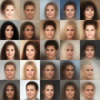
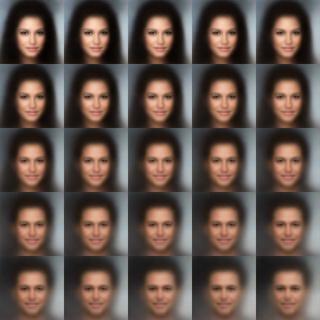
After training the model for some time on the CelebA dataset, I obtain the following results (reconstructions, samples and interpolation). 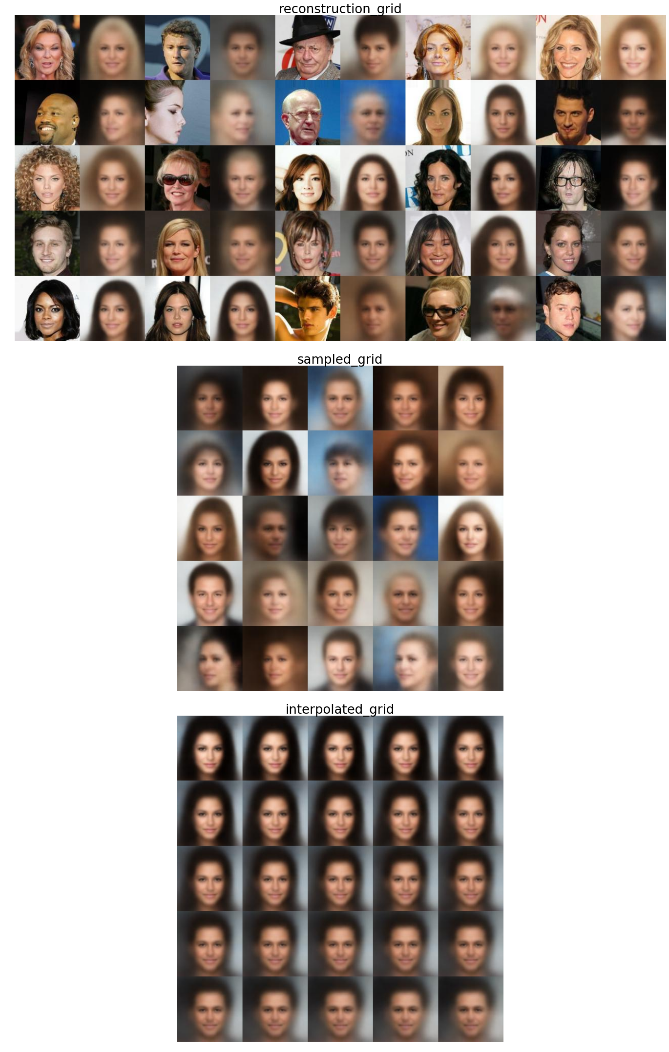
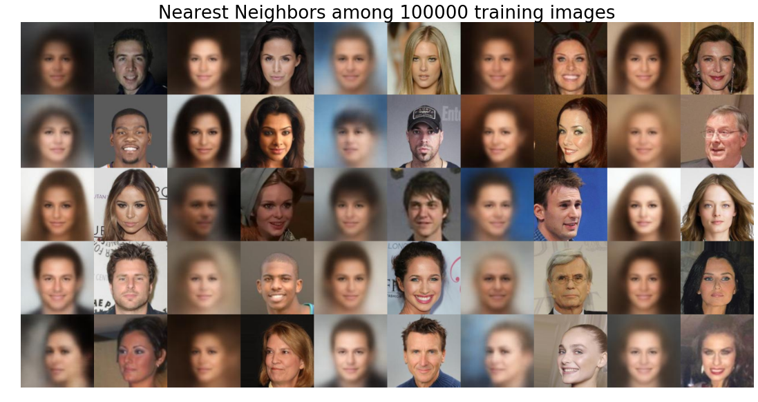
As is typical for VAEs under a Gaussian assumption, the resulting samples are rather blurry. However the model is able to generate new unseen samples. In fact, we can search for the nearest neighbors of the generated images in the training set (in terms of L2 distance), to check for any potential overfitting problems (which does not seem to be the case here):