This post is a short introduction and Python implementation of the Delaunay and Alpha Complexes triangulation in 2D. For additional reference, see for instance Computational Topology: An Introduction, H. Edelsbrunner and J. Harer, Chapter 3, Section 4.
Introduction
Mesh generation is the problem of generating a mesh composed of polygons (or polyhedrons in higher dimensions) from a cloud of points. This has typical applications for instance in Computer Graphics, when one wants to produce a model of a surface matching a given point cloud. In particular, an interesting issue is how well the generated mesh respect the original shape that the point cloud is induced from. This obviously depends on the cloud density, but also on the meshing algorithm used.
In this post, I will focus on the 2D case for simplicity and introduce Delaunay Triangulation and Alpha Complexes for mesh generation. We will see that Alpha Complexes are a subset of the Delaunay Triangulation and that they are able to preserve topological information from the initial shape: Contrary to the Delaunay triangulation, it can generates meshes with holes thanks to a radius constraint.
Basics: The convex hull
Point cloud generation
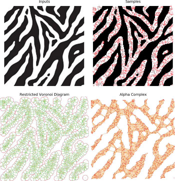
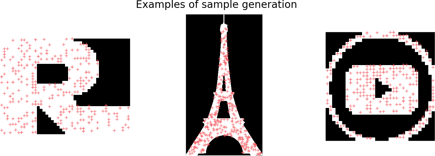
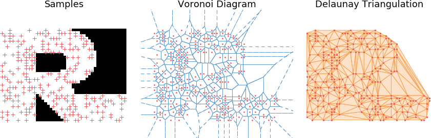
In the rest of this post, I will use point clouds generated by randomly sampling the space defined by a binary mask as inputs. In particular we will consider shapes displaying various topological content (i.e. in the 2D contents, different numbers of holes and connected components)
def generate_cloud_from_image(N, image):
    # Threshold
    image[image > 125] = 255
    image[image < 125] = 0

    # Sample from the white pixels
    indices = np.random.choice(np.where(image.flatten() != 0)[0], size=N)
    samples = np.zeros((N, 2))
    samples[:, 0] = indices % image.shape[1]
    samples[:, 1] = indices / image.shape[1]
The convex hull
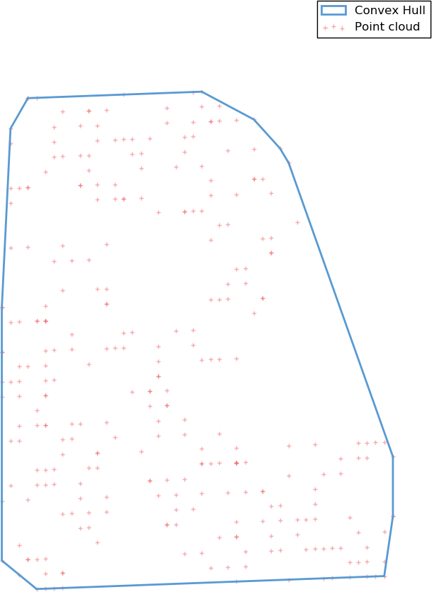
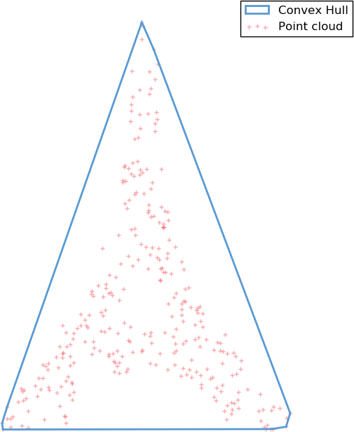
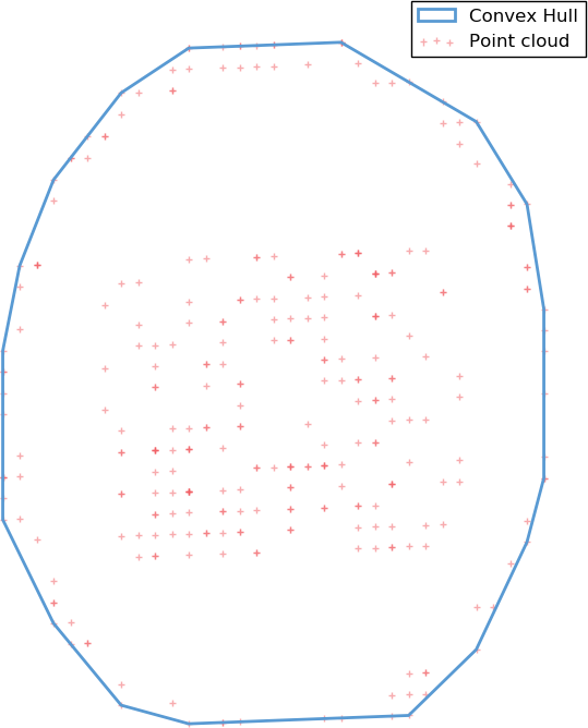
A first possible very simple meshing algorithm is to take the convex hull of the points cloud. The convex hull of a point set is simply the tightest convex set that contains the whole set. While simple to build, this model is heavily constrained by the convex requirement, and is a bad approximation for any shape displaying non-convex features.
The Delaunay triangulation
Definition
A triangulation of a 2D point cloud \(S \in \mathbb{R}^2\) is triangulation of its convex hull, i.e. a partition of the hull in triangles whose vertices are points of \(S\). Additionally, a Delaunay triangulation \(DT(S)\) is such that no points in \(S\) is inside any of the circumscribed circles to any of the triangles in \(DT(S)\), which guarantees a certain regularity to it; In particular it typically prevents very elongated triangles.
Note: According to the definition, the Delaunay Triangulation also has a limiting convex constraint. In order to avoid this, a classical trick is to had some boundary points to form a bounding box around the point clouds, forming a new convex hull. Then after the triangulation is done, we simply remove the triangles for which any vertex lies on the boundary. That way, we retrieve a potentially non-convex triangulation of the original point cloud \(S\).
Voronoi Diagram
An easy to compute the Delaunay triangulation is to characterize it as the dual of the Voronoi diagram of \(S\). More specifically, for each point \(x \in S\), its Voronoi cell is defined as the set of points in the space which are closer to \(x\) than any other points in \(S\): \begin{align} V_x = \left[ y \in \mathbb{R}^2,\ \mbox{s.t. } \forall x’ \in S,\ || y - x||_2 \leq ||y - x’||_2 \right] \end{align}
def voronoi_diagram(samples, ax=None):
    # Extract Voronoi regions (sicpy)
    vor = Voronoi(samples, qhull_options="Q0")

    # vor_ridges; Maps edge index -> Center of incident Voronoi cells
    n = len(vor.vertices)
    vor_ridges = {min(edges) * n + max(edges):
                  ((centers[0], vor.points[centers[0]]),
		   (centers[1], vor.points[centers[1]]))
                  for edges, centers in zip(vor.ridge_vertices, vor.ridge_points)}
Building the triangulation
Finally, the Delaunay triangulation is built as the dual of the Voronoi diagram, i.e. we form an edge between any two points \(x, x' \in S\) if and only if their respective cells \(V_x\) and \(V_{x'}\) touch (have a common edge) in the Voronoi diagram.
\begin{align} DL(S): x \leftrightarrow x’ \iff V_x \mbox{ adjacent to } V_{x’} \end{align}
# Build vertices and triangles list
adjacency = defaultdict(lambda: [])
vertices = {}
for (ip, p), (iq, q) in vor_ridges.values():
    vertices[ip] = p
    vertices[iq] = q
    adjacency[min(ip, iq)].append(max(ip, iq))

# Build triangles for adjacent cells
triangles = []
for p, neighbours in adjacency.items():
auxp = set(adjacency[p])
for i, q in enumerate(neighbours):
    auxq = auxp & (set(adjacency[q]))
    for r in neighbours[i+1:]:
        if max(q,r) in adjacency[min(q, r)] and
           len(list(auxq.intersection(adjacency[r]))) == 0:
            triangles.append(mp.Polygon(
		[vertices[p], vertices[q], vertices[r]], closed=True))
Alpha Complexes
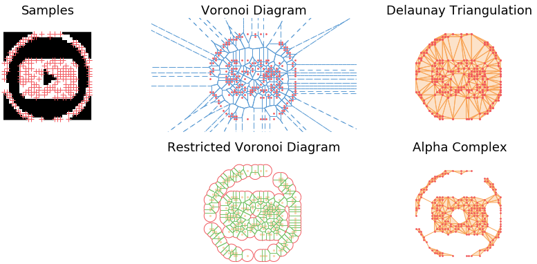
As we have seen in the previous example, the Delaunay triangulation yields a much more interesting result shape than the convex hull. However, it produces a dense partition of the space and in particular doesn’t recover topological information from the shape such as holes or connected components.
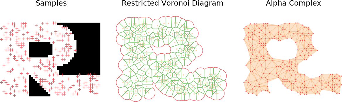
Alpha complexes are a subset of the Delaunay Triangulation that tackles this issue. As previously, we will use a dual structure. More specifically, Alpha complexes are defined as the dual construction of the restricted Voronoi diagram, \(Vor_r(S)\). Which is simply the intersection of the Voronoi diagram with balls of radius \(r\) centered on every point in \(S\).
\begin{align} Vor_r(S) = \left[ V_x \cap B_{r}(x),\ \forall x \in S \right] \end{align}
Line-circle intersection
In order to build the restricted Voronoi diagram, we need to start from the initial Voronoi diagram and compute its intersections with balls of radius \(r\). In 2D, this means we need to compute intersections between circles and the lines composing the diagram.
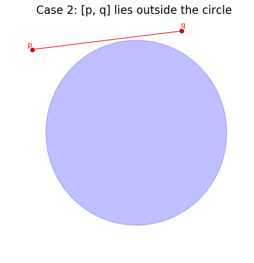
The first two easy cases are when the line segment of the diagram, [p, q] is fully inside or fully outside the circle.
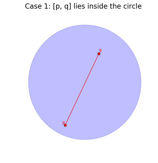
# Case 1: If p and q are both in the circle -> clip to [p, q]
if is_in_circle(p, center, r) and is_in_circle(q, center, r):
return [(p, q)], True, True

# Intersection with line y = ax + b
# Express the line equation as y = slope * x + intersect
slope = (q[1] - p[1]) / (q[0] - p[0])
intersect = q[1] - slope * q[0]
# Express the intersection problem as a quadratic equation ax2 + bx + c
# we need to solve the system:
#   (1) y = slope  * x + b
#   (2) (x - center[0])**2 + (y - center[1])**2 = r
a = slope**2 + 1
b = 2 * (slope * (intersect - center[1]) - center[0])
c = center[0]**2 + (intersect - center[1])**2 - r**2

# Case 2: No intersection
delta = b**2 - 4*a*c
if delta <= 0:
    return [], False, False
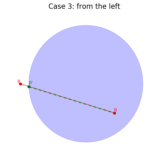
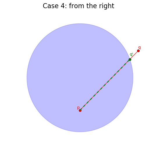
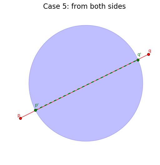
When the segment does intersect with the circle, we need to take into consideration whether it intersects from the “left”, from the “right” or from both sides (here we order the segment extremities by increasing order of their x-coordinate).
# Intersection -> clip to [p2, q2] n [p, q]
else:
pt1 = p; pt2 = q
is_in_pq = lambda z: (z >=  p[0]) and (z <= q[0])
check = False # check will be True iff [p2, q2] n [p, q] is empty

# Case 3: p is not in the circle
if not is_in_circle(p, center, r):
    x = (- b - np.sqrt(delta)) / (2 * a)
    pt1 = np.array([x, slope*x + intersect])
    check = not is_in_pq(x)

# Case 4: q is not in the circle
if not is_in_circle(q, center, r):
    x = (- b + np.sqrt(delta)) / (2 * a)
    pt2 = np.array([x, slope*x + intersect])
    check = (check or cp) and (not is_in_pq(x))

# Case 5: neither p or q are inside the circle
return ([], False, False) if check else
    ([(pt1, pt2)],  is_in_circle(p, center, r),  is_in_circle(q, center, r))
Building the restricted Voronoi diagram
Once we have this construction, we can build the restricted Voronoi Diagram. We consider every segment \([p, q]\) of the Voronoi diagram. Let us denote \(V_x\) and \(v_y\) the two Voronoi cells that lie on both sides of \([p, q]\); we say \([p, q]\) is a ridge between \(V_x\) and \(V_y\).
We need to compute the intersections between \([p, q]\) and \(B(x, r)\) (or equivalently, \(B(y ,r)\), since by definition of the Voronoi diagram, any point on the ridge is equidistant from \(x\) and \(y\)). A restricted Voronoi cell is represented as a sequence of edges \([(p_0, q_0), \dots (p_n, q_n)]\), where \([p_i, q_i]\) is a segment. Furthermore, either \(q_i = p_{i + 1}\), or \(q_i \neq p_{i + 1}\) in which case \(q_i\) and \(p_{i + 1}\) are joint by a circle segment.
for center, region, region_indices, edge_indices in vor_regions:
    restr_region = []
    for i, p in enumerate(region):
        q = region[(i + 1) % len(region)]
        inter, clip_p, clip_q = line_circle_intersection(p, q, center, r)
        restr_region.extend(inter)
        restricted_voronoi_cells.append((center, restr_region))
Building the alpha complex
Building the alpha complex from the restricted Voronoi diagram is straightforward. We will split it in two sets: the triangles, which are triangles of the Delaunay triangulation and occur whenever a point lying at the intersection of three Voronoi cells still exist in the restricted Voronoi diagram (i.e. if it belongs to one the balls of radius \(r\)). The second set are the edges and are the leftover edges which still exist in the alpha complex but are not part of a full triangle due to the radius constraint.
    ... # continued
    if clip_p:
        triangles[region_indices[i]].append(edge_indices[i])
    if clip_q:
        triangles[region_indices[(i + 1) % len(region)]].append(edge_indices[i])
    else:
        alpha_complex_cells[0].append(edge_indices[i])

# Form triangles
for vertex, incident_edges in triangles.items():
if len(incident_edges) == 3:
    vertices = [(x, y) for e in incident_edges for (x, y) in vor_ridges[e]]
    _, aux = np.unique([x[0] for x in vertices], return_index=True)
    alpha_complex_cells[1].append([vertices[i][1] for i in aux])
Demo
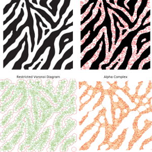
The main observation is that by tuning the radius constraint correctly, we can obtain a mesh of the point clouds that respect topological features of the original shape (holes), contrary to the Delaunay Triangulation. However, finding a good value for this parameter can be quite difficult as it heavily depends on the input samples.
To highlight this, I also generate an animation of the restricted Voronoi diagram and the alpha complex for growing value of \(r\). For very small \(r\), no cells collide and the complex is equal to the point cloud; Inversely for large \(r\), the complex collapses to the Delaunay Triangulation. For values in between, we get different density meshes of the cloud.