The Pólya Urn

The Pólya urn model is a statistical experiment in which we study the distribution of two populations of distinctly colored balls in an urn. In its simplest form, the problem can be stated as follows:

This process is a good example of a model where small imbalances are magnified over time: In fact, the more balls of one color are drawn, the more this color is likely to be drawn. As such, it has been used to model for instance propagation of epidemics in a population (Hayhoe et al.) or the correlated dynamics between novelty events (Tria et al, 2014). In the following, we study the dynamics of the model from a probabilistic point of view and its asymptotical properties, in particular with respect to the initial ratio of populations.

Basic dynamics of the model

Composition of the urn at step n

Let us first express the probability of having picked $k$ blue objects after $n \geq k$ steps of the experiment. Denoting by $B_n$ the number of blue balls at step $n$ , and by $S_n$ the sampling event at step $n$ , taking value 1 if a blue ball is sampled and 0 otherwise:

We can expand the inner term by using the probability chain rule. Moreover, the probability of drawing a ball of a certain color given the composition of the urn is simply the ratio of correspondingly colored balls in the urn, which evolves with each sampling. Therefore, the conditional probability of drawing a blue object at step $n$ can be written as:

From this expression, we can see that the probability does not depend on the time step $n$ but rather on how many blue balls have been sampled until now, as captured by the quantity $\sum_{i=1}^{n-1} s_i$ . This also means that the model is Markovian, as the probability at step $n$ only depends on the urn’s composition at step $n - 1$ .

Consequently, for any sequence of draws $\mathbf{s}$ , we can arrange the order in which the balls have been drawn without affecting the probability of the next draw. This is sometimes called the exchangeability property. More formally, it means that Equation (1) is equivalent to:

where $\bar{\mathbf{s}}$ is a shortcut notation for $\sum_{i=1}^{n-1} s_i$ from $(1)$ . The same analysis holds for the conditional probability of drawing an orange ball. Bringing everything together, we can thus finally write $\mathbb{P} (B_n = b + k) = \binom{n}{k} \mathbb{P}(S_1 = \textcolor{CornflowerBlue}{1}, \dots, S_k = \textcolor{CornflowerBlue}{1}, S_{k+1} = \textcolor{Orange}{0} \dots S_{n} = \textcolor{Orange}{0})$

Probability of the next draw

Following the previous result, we can now compute the probability of picking a blue ball at step $n + 1$ , independently of the state of the urn at time $n$ :

To simplify the expression of $f(n, a, b)$ , we can use Pascal’s triangle formula on the numerator (while isolating the terms for $j = 0$ and $j = n$ ) and observe that: $f(n, a, b) = \sum_{j=0}^n \frac{\binom{n}{j}}{\binom{a+b+n-1}{b+j}}$

By extending the relation, one can infer and finally prove by induction over $n$ , that $f(n, a, b) = \frac{a+b+n}{(a+b) \binom{a+b-1}{b}}$ . Plugging this expression in Equation (3), we finally get:

In other words, the overall probability of the urn composition after $n$ only depends on the initial color distribution in the urn. In particular, for the case where $a = 1$ and $b = 1$ we have $\mathbb{P} (B_n = k + 1) = \frac{[\!|\ k \leq n \ |\!]}{n + 1}$ and $\mathbb{P} (S_n = 1) = 0.5$ . In other words, all urn configurations are equiprobable when starting from a balanced urn.

Asymptotic behavior

Expected value

Since various urn compositions can be reached from the same initial configuration ( $a$ , $b$ ), one can also wonder what the urn composition looks like asymptotically, when the number of repeats $n$ goes to $\infty$ .

Let us introduce $Y_n = \frac{B_n}{a + b +n}$ , the ratio of the two colored ball populations at step $n$ . Using the previous results, we can easily see that the expected value of $Y_n$ is equal to the initial ratio, independently of the time step:

This can also be observed in simulations. Here, blue lines ( --- ) represent the observed value of $Y_n$ for each time step $n \leq$ 100 for 70 different runs with the same initial conditions $a$ and $b$ . Red circles ( ● ) mark the average of these values across runs, for each time step, hence serve as an approximation of $\mathbb{E}(Y_n)$ .

Link to the Dirichlet-multinomial distribution

Going further, we can also study the convergence in distribution of the random variable $Y_n$ . First we observe that the probability distribution of $Y_n$ is directly linked to the one of $B_n$ , that we expressed earlier.

We can further simplify the expression by making use of the Gamma and Beta functions. This yields the following result:

Where the Gamma and Beta functions are defined as $\Gamma: x \mapsto (x - 1)!$ and $\beta: (a, b) \mapsto \frac{\Gamma(a)\Gamma(b)}{\Gamma(a+b)} = \int_0^1 x^{a-1} (1-x)^{b-1}dx$ respectively.

Note that, up to a simple rearrangement of terms in Equation (4), we observe that $Y_n$ follows a Dirichlet-multinomal distribution with parameters $\alpha = (a, b)$ . And in fact, this distribution is also known as the multivariate Pólya distribution and can be generalized to urns with more than two color populations.

Asymptotic distribution

To prove a convergence in distribution, we want to look at the limit of the repartition function of $Y_n$ , defined as $F_{Y_n}(x) = \mathbb{P}(Y_n \leq x)$ , when the time step $n \rightarrow \infty$ . Using the previous simplified expression, we have:

Thus $g(x,t,n, a, b)$ is the only term that depends on $n$ . Its expression is clearly linked, and similar to, a binomial expansion: More specifically, if we define the random variable $X_n$ with a binomial distribution of parameters $n$ and $x \in [0, 1]$ , then we have exactly that $g(x, t, n, a, b) = \mathbb{P}(X_n \leq t(a+b+n) - b)$ .

We can then directly apply the Demoivre-Laplace theorem, which derives from the Central Limit theorem, to $X_n$ which yields that, for large $n$ ,

where $\Phi$ is the repartition function of the standard Gaussian distribution, $\mathcal{N}(0,1)$ , and, as such, is continuous and bounded. As a result, we have that:

By splitting the integral from Equation (5) at point $t \in [0, 1]$ , we conclude that

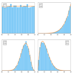
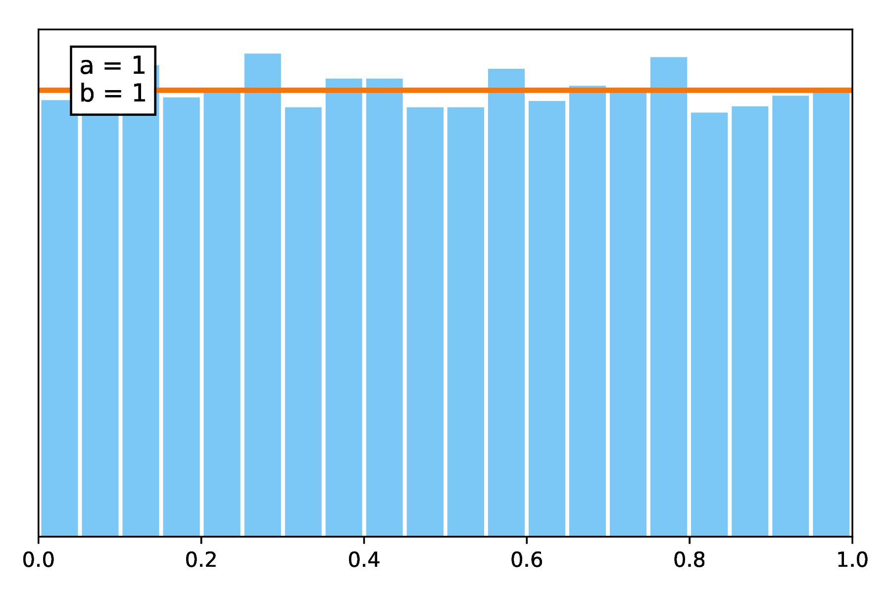
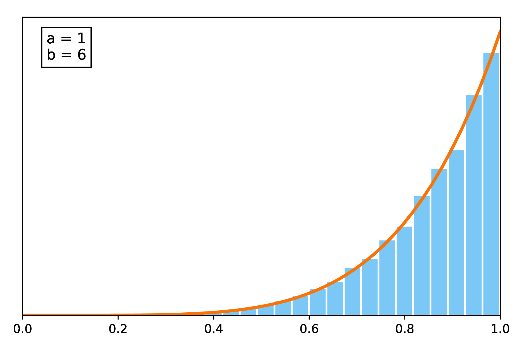
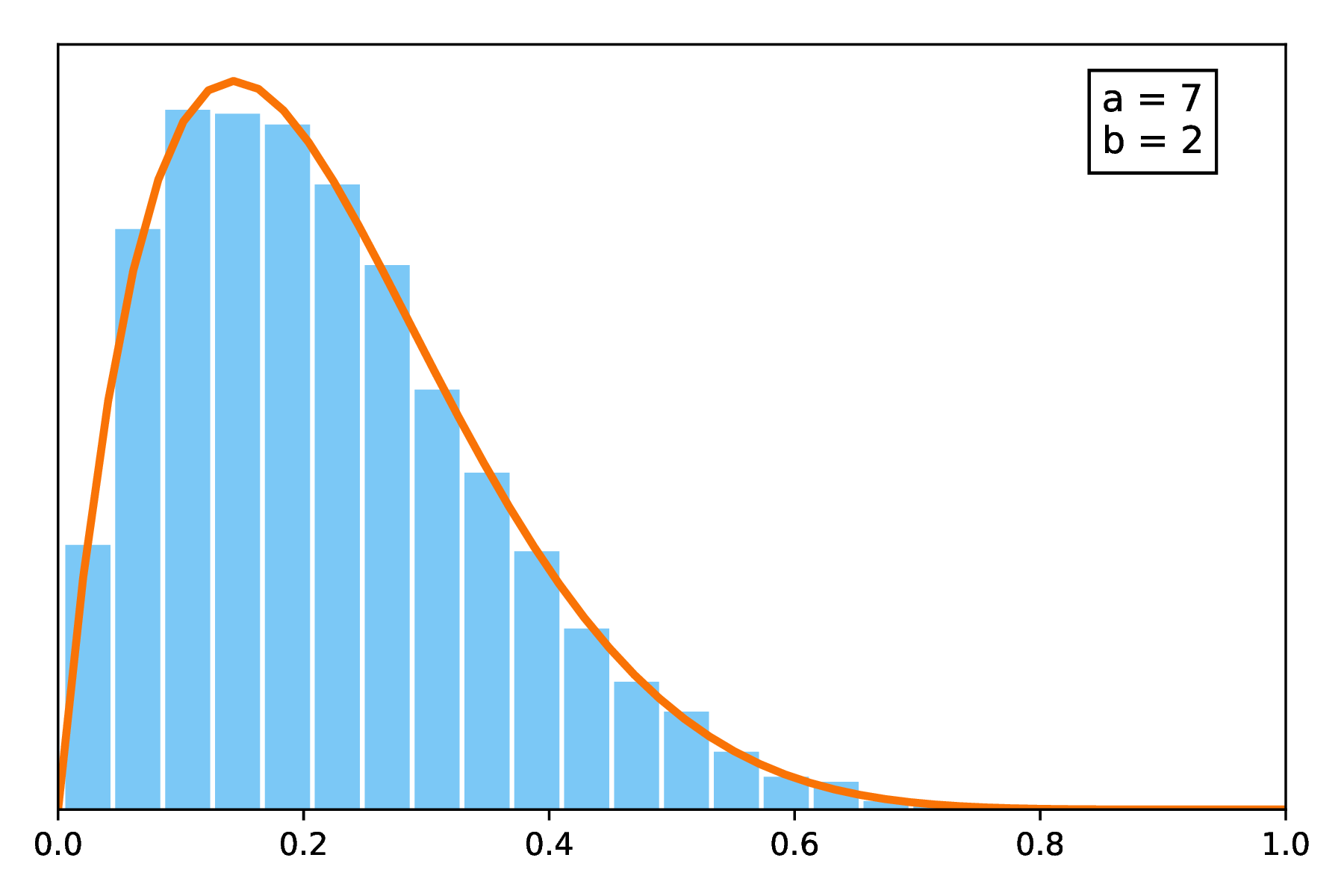
The right-side term is exactly the repartition function of a Beta distribution at point $t$ . Thus, the proportion of blue balls in the urn, $Y_n$ , converges in distribution to the Beta distribution with parameters b and a when $n$ grows.

Figure 3: Histograms of observed values of $Y_{n = 1000}$ for 10000 runs with different initial conditions (a , b), compared to the density function of the $\beta(b, a)$ distribution (represented as --- ).

Generalized Pólya urn

We won’t study such models here, but it is possible to extend the Pólya urn experiment to more flexible frameworks: Generalized Pólya urns follow the same workflow as the one we have been working with until now, but with different replacement values. More specifically, the experiment is described as follows:

Such a model is often represented by its initial conditions (a , b), and its replacement matrix, $R = \begin{pmatrix} \alpha & \beta \\ \gamma & \delta \end{pmatrix}$ .

It is also possible to generalize the urn to an arbitrary number of colors, leading to a $d \times d$ replacement matrix. For instance, in the standard Pólya setting, we have $d = 2$ and $R = \begin{pmatrix} 1 & 0 \\ 0& 1 \end{pmatrix} = I_2$

References

• “A Pólya Contagion Model for Networks”, M. Hayhoe et al, 2017
• “A survey of random processes with reinforcement”, R. Pemantle, 2017
• “On generalized Pólya urn models”, M. Chen and M. Kuba, 2011
• “Pólya urn models: Lecture Notes”, N. Pouyanne, 2004
• “Rate of convergence of Pólya’s urn to the Beta distribution”, J. Drinane, 2008
• ″The dynamics of correlated novelties”, F. Tria et al, 2014
• “Urnes aléatoires, populations en équilibre et séries génératrices”, B. Mallein, 2010