Generative Latent Optimization
October 12, 2017
This post contains a short introduction and Tensorflow v1 (graph-based) implementationof the Generative Latent Optimization (GLO) model as introduced in Optimizing the Latent Space of Generative Networks, P. Bojanowski, A. Joulin, D. Lopez-Paz, A. Szlam, ICLR 2017.
Model
Comparison to Variational Auto Encoders
In the context of Variational Autoencoders (see this previous post), the GLO model can be seen as a VAE without an encoder, where the latent codes are free variables learned directly from the data. This considerably simplifies the model at training time, as we simply optimize the latent codes and the variables of the decoder based on a reconstruction loss.
On the other hand, inference is ill-posed, as we do not have an explicit prior to sample codes from, contrary to the VAE setting. In order to palliate this problem, the GLO paper proposes to constrain the space of latent codes by projecting them to the unit ball. Images are then generated by sampling new codes either from a unit variance Gaussian, or from a diagonal covariance Gaussian fitted to the codes learned from the training set.
Formal definition
Formally, at training time, given an input image , the model produces a reconstruction where is a random variable on the unit ball and is a decoder network. The model is trained by minimizing the reconstruction loss between and respectively to the variables and the parameters of the decoder .
At inference time, we can define a prior either as an arbitrary distribution (e.g., unit variance Gaussian), or by fitting a parametric distribution to the training samples latent codes.
Implementation
Inputs pipeline
First, we define the input pipeline as queue which contains images from a given list of filenames and a unique integer identifier for each.
The get_inputs_queue function returns a queue whose elements are input dictionary with keys:
- image: A 4D Tensor of size (batch_size, height, width, num_channels) representing the input images.
- index: A scalar Tensor containing the index of the image in the database
# Read index (no shuffle)
index_queue = tf.train.range_input_producer(
    len(filenames), capacity=capacity, shuffle=False)
inputs['index'] = index_queue.dequeue()

# Read Image (no shuffle so same order as index)
filename_queue = tf.train.string_input_producer(
    filenames, capacity=capacity, shuffle=False)
_, reader = tf.WholeFileReader().read(filename_queue)
inputs['image'] = image

# Preprocess the inputs
with tf.variable_scope('inputs_preprocess'):
    inputs = preprocess_inputs(inputs)

# Batch the inputs
inputs = tf.train.shuffle_batch(
   inputs, batch_size, capacity, min_after_dequeue)
Architecture
As mentionned, there is no encoder in GLO. We directly learn the code as a free variable for each input training image , without imposing a parametric form of the latent code distribution. In particular, this implies that the number of variables grows linearly with the number of data samples.
Additionally, the code space is constrained by projecting each code to the unit ball before feeding them to the decoder.
def project(z):
   return z / tf.sqrt(tf.reduce_sum(z ** 2, axis=1, keep_dims=True))
For the decoder, I used a simple convolutional architecture with ReLU activations and batch normalization layers.
- Inputs: (batch, num_latent_dims)
- 1 deconvolution upscale the input to (batch, 4, 4, c)
- 5 deconvolutional blocks
- transpose convolution, stride 2, kernel size 3
- ReLU activation and Batch normalization
- Outputs: (batch, 128, 128, 3)
with tf.variable_scope('decoder', reuse=reuse):
   with slim.arg_scope([slim.conv2d_transpose], stride=2,
                        weights_initializer=weights_initializer,
                        activation_fn=activation_fn,
                        normalizer_fn=normalizer_fn,
                        normalizer_params=normalizer_params,
                        padding='SAME'):
        # Flattened input -> 4 x 4 patch
        shape = latent_z.get_shape().as_list()
        net = tf.reshape(latent_z, (shape[0], 1, 1, shape[1]))
        net = slim.conv2d_transpose(net, num_filters[0], [4, 4], stride=1,
                                    padding='VALID', scope='deconv1')

        # Upscale via deconvolutions
        for i, num_filter in enumerate(num_filters[1:]):
            net = slim.conv2d_transpose(net, num_filter,
	    	  			[kernel_size, kernel_size],
                                        scope='deconv%d' % (i + 2))

        # Final deconvolution
        net = slim.conv2d_transpose(net, 3, [3, 3], stride=2,
                                    activation_fn=tf.nn.tanh,
                                    normalizer_fn=None,
                                    scope='deconv_out')
Loss function
Finally as mentionned previously, the loss function reduces to a simple reconstruction loss term between the input and reconstructed images (here we use a simple mean squared error).
def get_glo_loss(images, reconstructions, weight=1.0):
    return weight * tf.reduce_mean(tf.square(images - reconstructions))
Training
We’re now ready for training. During training, the latent codes are directly optimized and are stored as trainable Tensorflow variables in codes, that can be retrieved by slicing with the corresponding index. Due to the large size of the dataset (~ 200k samples in CelebA), the model requires a few epochs before starting to learn reasonable codes.
with tf.Graph().as_default():
    ## latent codes
    codes = slim.variable('codes', dtype=tf.float32,
                          shape=(len(filenames), NUM_DIMS),
                          trainable=True)

    ## Training Network
    for i in range(NUM_GPUS):
        # inputs
        with tf.name_scope('inputs_%d' % (i + 1)):
            inputs = get_inputs_queue(BASE_DIR, batch_size=BATCH_SIZE)

        # outputs
        outputs = {}
        with tf.name_scope('model_%d' % i):
            with tf.device('/gpu:%d' % i):
                # retrieve code
                outputs['code'] = tf.gather(codes, inputs['index'])

                # project code
                outputs['code'] = project(outputs['code'])

                # decode
                outputs['reconstruction'] = decoder(
                    outputs['code'],
                    num_filters=NUM_DECODER_FILTERS,
                    reuse=i > 0)

        # loss
        with tf.name_scope('loss_%d' % i):
            loss =  tf.losses.mean_pairwise_squared_error(
                inputs['image'], outputs['reconstruction'])

    # Optimization
    global_step = tf.contrib.framework.get_or_create_global_step()
    optimizer = tf.train.AdamOptimizer(learning_rate=LEARNING_RATE)
    loss = tf.add_n(tf.get_collection('total_loss')) / NUM_GPUS
    train_op = optimizer.minimize(loss, global_step=global_step,
                                  colocate_gradients_with_ops=True)

    # Update op for batch norm
    update_ops = tf.get_collection(tf.GraphKeys.UPDATE_OPS)
    train_op = tf.group(train_op, *update_ops)

    ## Launch the training session
    try:
        with get_monitored_training_session() as sess:
            global_step_,loss_, _ = sess.run([global_step, loss, train_op])
            print('\rStep %d: %.3f' % (global_step_, loss_), end='')
    except KeyboardInterrupt:
        print('\nInterrupted at step %d' % global_step_)
Results
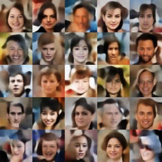
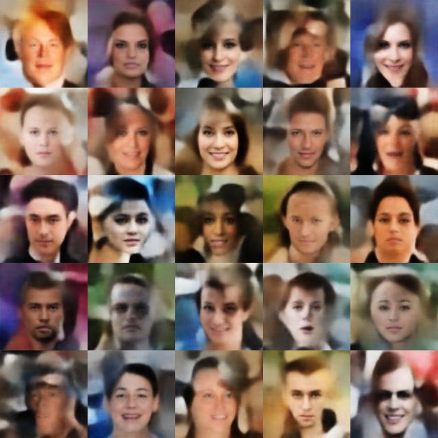
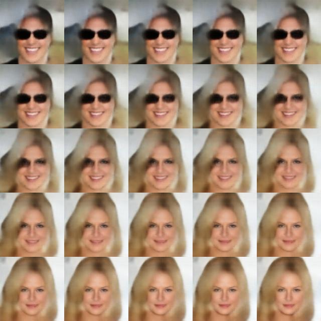
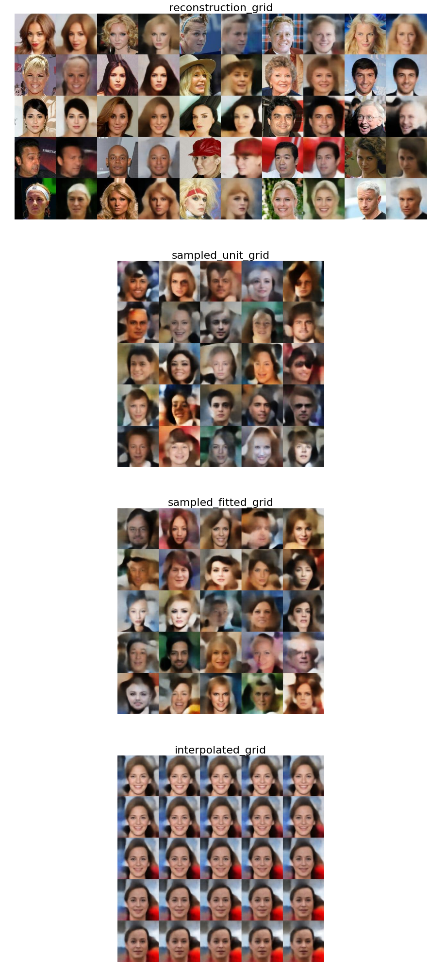
After training the model for some time on the CelebA dataset, I obtain the following results (reconstructions, samples and interpolation). Now that the latent code distribution is not constrained, the samples are visually crisper than the ones generated from a vanilla VAE. However the sampling process is not as well justified.
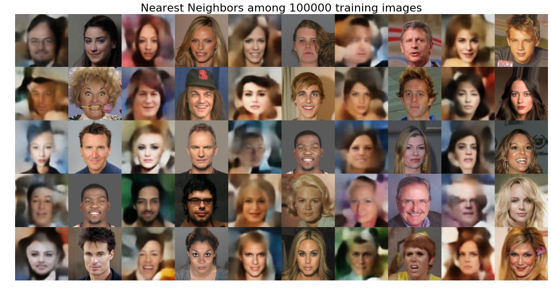
We also observe that the model does not seem to overfit to the training dataset and is able to generate unseen samples. See for instance the result of nearest neighbor search across the training dataset: