This notebook contains a Keras / Tensorflow implementation of the VQ-VAE model, which was introduced in Neural Discrete Representation Learning (van den Oord et al, NeurIPS 2017). This is a generative model based on Variational Auto Encoders (VAE) which aims to make the latent space discrete using Vector Quantization (VQ) techniques. This implementation trains a VQ-VAE based on simple convolutional blocks (no auto-regressive decoder), and a PixelCNN categorical prior as described in the paper. The current code was tested on MNIST. This project is also hosted as a Kaggle notebook.
Pros (+)
- Simple method and training objective
- “Proper” Discrete latent space. This is a promising property to model data that is inherently discrete, e.g. text.
Cons (-)
- Loses the “easy latent sampling” property from VAEs. Two-stage training required to learn a fitting categorical prior.
- The training objective does not correspond to a bound on the log-likelihood anymore.
Vector-Quantized Latent Space
The first step is to build the main VQ-VAE model. It consists of a standard encoder-decoder architecture with convolutional blocks. The main novelty lies in the intermediate Vector Quantizer layer (VQ) that takes care of building a discrete latent space.
More specifically, the encoder, \(f\), is a fully-convolutional neural network that maps input images to latent codes of size \((w, h, d)\), where \(d\) is the dimension of the latent space, and \(w \times h\) the size of the final feature map. The output of the encoder is then mapped to the closest entry in a discrete codebook of \(K\) latent codes, \(\mathcal E = \{e_0 \dots e_{K-1} \}\) where \(\forall i, e_i \in \mathbb{R}^d\).
\[\begin{align} &\textbf{input }x \tag{W x H x C}\\ z_e &= f(x) \tag{w x h x d}\\ z_q^{i, j} &= \arg\min_{e \in \mathcal E} \| z_e^{i, j} - e \|^2 \end{align}\]The Vector Quantization process is implemented as the following Keras layer:
class VectorQuantizer(K.layers.Layer):
    def __init__(self, k, **kwargs):
        super(VectorQuantizer, self).__init__(**kwargs)
        self.k = k

    def build(self, input_shape):
        self.d = int(input_shape[-1])
        rand_init = K.initializers.VarianceScaling(distribution="uniform")
        self.codebook = self.add_weight(shape=(self.k, self.d), initializer=rand_init, trainable=True)

    def call(self, inputs):
        # Map z_e of shape (b, w,, h, d) to indices in the codebook
        lookup_ = tf.reshape(self.codebook, shape=(1, 1, 1, self.k, self.d))
        z_e = tf.expand_dims(inputs, -2)
        dist = tf.norm(z_e - lookup_, axis=-1)
        k_index = tf.argmin(dist, axis=-1)
        return k_index

    def sample(self, k_index):
        # Map indices array of shape (b, w, h) to actual codebook z_q
        lookup_ = tf.reshape(self.codebook, shape=(1, 1, 1, self.k, self.d))
        k_index_one_hot = tf.one_hot(k_index, self.k)
        z_q = lookup_ * k_index_one_hot[..., None]
        z_q = tf.reduce_sum(z_q, axis=-2)
        return z_q
The decoder, \(g\), then takes the quantized codes \(z_q\) as inputs and generates the output image. Here we consider a simple architecture with transposed convolution blocks, mirroring the encoder architecture:
def encoder_pass(inputs, d, num_layers=[16, 32]):
    x = inputs
    for i, filters in enumerate(num_layers):
        x = K.layers.Conv2D(filters=filters, kernel_size=3, padding='SAME', activation='relu',
                            strides=(2, 2), name="conv{}".format(i + 1))(x)
    z_e = K.layers.Conv2D(filters=d, kernel_size=3, padding='SAME', activation=None,
                          strides=(1, 1), name='z_e')(x)
    return z_e

def decoder_pass(inputs, num_layers=[32, 16]):
    y = inputs
    for i, filters in enumerate(num_layers):
        y = K.layers.Conv2DTranspose(filters=filters, kernel_size=4, strides=(2, 2), padding="SAME",
                                     activation='relu', name="convT{}".format(i + 1))(y)
    decoded = K.layers.Conv2DTranspose(filters=1, kernel_size=3, strides=(1, 1),
                                       padding="SAME", activation='sigmoid', name='output')(y)
    return decoded
Once these three building blocks are done, we can build the full VQ-VAE. One subtility is how we can estimate gradient through the Vector Quantizer: In fact, the transition from \(z_e\) to \(z_q\) does not allow to backpropagate gradient due to the argmin function. Instead, the authors propose to use a straight-through estimator, that directly copies the gradient received by \(z_q\) to \(z_e\).
def build_vqvae(k, d, input_shape=(28, 28, 1), num_layers=[16, 32]):
    global SIZE
    ## Encoder
    encoder_inputs = K.layers.Input(shape=input_shape, name='encoder_inputs')
    z_e = encoder_pass(encoder_inputs, d, num_layers=num_layers)
    SIZE = int(z_e.get_shape()[1])

    ## Vector Quantization
    vector_quantizer = VectorQuantizer(k, name="vector_quantizer")
    codebook_indices = vector_quantizer(z_e)
    encoder = K.Model(inputs=encoder_inputs, outputs=codebook_indices, name='encoder')

    ## Decoder
    decoder_inputs = K.layers.Input(shape=(SIZE, SIZE, d), name='decoder_inputs')
    decoded = decoder_pass(decoder_inputs, num_layers=num_layers[::-1])
    decoder = K.Model(inputs=decoder_inputs, outputs=decoded, name='decoder')

    ## VQVAE Model (training)
    sampling_layer = K.layers.Lambda(lambda x: vector_quantizer.sample(x), name="sample_from_codebook")
    z_q = sampling_layer(codebook_indices)
    codes = tf.stack([z_e, z_q], axis=-1)
    codes = K.layers.Lambda(lambda x: x, name='latent_codes')(codes)
    straight_through = K.layers.Lambda(lambda x : x[1] + tf.stop_gradient(x[0] - x[1]), name="straight_through_estimator")
    straight_through_zq = straight_through([z_q, z_e])
    reconstructed = decoder(straight_through_zq)
    vq_vae = K.Model(inputs=encoder_inputs, outputs=[reconstructed, codes], name='vq-vae')

    ## VQVAE model (inference)
    codebook_indices = K.layers.Input(shape=(SIZE, SIZE), name='discrete_codes', dtype=tf.int32)
    z_q = sampling_layer(codebook_indices)
    generated = decoder(z_q)
    vq_vae_sampler = K.Model(inputs=codebook_indices, outputs=generated, name='vq-vae-sampler')

    ## Transition from codebook indices to model (for training the prior later)
    indices = K.layers.Input(shape=(SIZE, SIZE), name='codes_sampler_inputs', dtype='int32')
    z_q = sampling_layer(indices)
    codes_sampler = K.Model(inputs=indices, outputs=z_q, name="codes_sampler")

    ## Getter to easily access the codebook for vizualisation
    indices = K.layers.Input(shape=(), dtype='int32')
    vector_model = K.Model(inputs=indices, outputs=vector_quantizer.sample(indices[:, None, None]), name='get_codebook')
    def get_vq_vae_codebook():
        codebook = vector_model.predict(np.arange(k))
        codebook = np.reshape(codebook, (k, d))
        return codebook

    return vq_vae, vq_vae_sampler, encoder, decoder, codes_sampler, get_vq_vae_codebook

vq_vae, vq_vae_sampler, encoder, decoder, codes_sampler, get_vq_vae_codebook = build_vqvae(
    NUM_LATENT_K, NUM_LATENT_D, input_shape=INPUT_SHAPE, num_layers=VQVAE_LAYERS)
vq_vae.summary()
Training the model
All is left now is to train the model: The training objective contains the reconstruction loss (here, we use mean squared error), the KL divergence term on the latent codebook (ignored because it is constant as we assume a uniform prior during training), and two vector quantization losses which guarantee that (i) the outputs of the encoder stay close to the codebook entries they are matched to and (ii) that the codebook does not grow too much relatively to the space of the encoder outputs.
\[\begin{align} \mathcal L_{\text{VQ-VAE}}(x) = - \mathbb{E}_{z \sim f(x)}{p(x | z)} + \| z_e - \bar{z_q}\|^2 + \|\bar{z_e} - z_q\|^2 \end{align}\]where \(\bar{\cdot}\) denotes the stop gradient operation: i.e., during forward pass, this corresponds to the identity, but during backpropagation no gradients are flowing through this operation.
def mse_loss(ground_truth, predictions):
    mse_loss = tf.reduce_mean((ground_truth - predictions)**2, name="mse_loss")
    return mse_loss

def latent_loss(dummy_ground_truth, outputs):
    global BETA
    del dummy_ground_truth
    z_e, z_q = tf.split(outputs, 2, axis=-1)
    vq_loss = tf.reduce_mean((tf.stop_gradient(z_e) - z_q)**2)
    commit_loss = tf.reduce_mean((z_e - tf.stop_gradient(z_q))**2)
    latent_loss = tf.identity(vq_loss + BETA * commit_loss, name="latent_loss")
    return latent_loss
We can now train the model on the MNIST dataset:
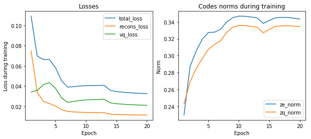
Figure 1: Training the VQ-VAE on the MNIST dataset
Once training is done, we can also visualize some of the results, such as reconstructions on the test set and the learned codebook entries (projected to 2D with TSNE). In particular, we observe that reconstructions are close to perfect, which indicates the model is able to learn a meaningful codebook, as well as how to map images to this discrete space.
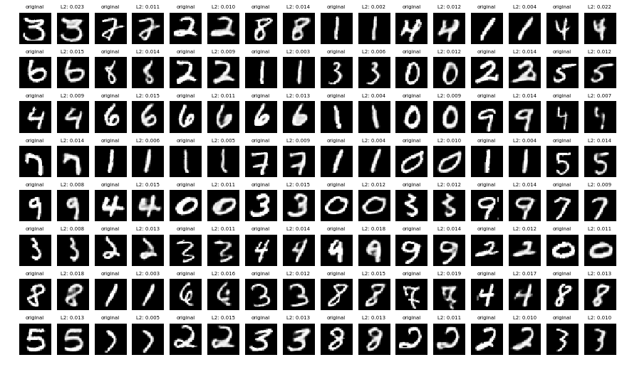
Figure 2: Reconstructions on the test set. The image reads row-wise such that every pair contains the original image (left) and its reconstruction (right) with the mean squared error distance to the original.
Learning a prior over the latent space
We have now learned an encoder-decoder architecture and a discrete latent codebook powerful enough to encode and reconstruct our dataset. However, the uniform prior assumption during training is not sufficient for generating good samples. In fact, due to the fully-convolutional architecture, each image is encoded with SIZE x SIZE latent vectors from the codebook (for instance, SIZE = 7 for our current model).
However, the codes for our dataset have no guarantee to lie uniformly on that space, as we assumed during training, but rather have some specific structure that follow a certain non-uniform categorical prior. This can be seen easily by generating images from code feature maps sampled uniformly from the total latent space of size SIZE x SIZE x \(K\).
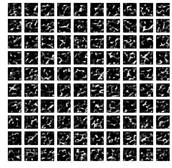
Figure 3: Generating samples from the uniform latent prior assumed during training
PixelCNN
To solve the problem and sample likely codes from the latent space, the authors propose to learn a powerful categorical prior over the latent codes from the training images using a PixelCNN. PixelCNN is a fully probabilistic autoregressive generative model that generates images (or here, feature maps) pixel by pixel, conditioned on the previously generated pixels. The main drawback of such models is that the sampling process is rather slow. However, since here we are only generating small SIZE x SIZE maps, the overhead is not too bad.
Here we consider the architecture proposed in Conditional Image Generation with PixelCNN Decoders (van den Oord et al, NeurIPS 2017) which uses gated and masked convolutions to model the fact that pixels only depend from the previously generated context. We implement the base building block of the architecture as the following Keras pipeline:
# References:
# https://github.com/anantzoid/Conditional-PixelCNN-decoder/blob/master/layers.py
# https://github.com/ritheshkumar95/pytorch-vqvae

def gate(inputs):
    """Gated activations"""
    x, y = tf.split(inputs, 2, axis=-1)
    return Kb.tanh(x) * Kb.sigmoid(y)


class MaskedConv2D(K.layers.Layer):
    """Masked convolution"""
    def __init__(self, kernel_size, out_dim, direction, mode, **kwargs):
        self.direction = direction     # Horizontal or vertical
        self.mode = mode               # Mask type "a" or "b"
        self.kernel_size = kernel_size
        self.out_dim = out_dim
        super(MaskedConv2D, self).__init__(**kwargs)

    def build(self, input_shape):
        filter_mid_y = self.kernel_size[0] // 2
        filter_mid_x = self.kernel_size[1] // 2
        in_dim = int(input_shape[-1])
        w_shape = [self.kernel_size[0], self.kernel_size[1], in_dim, self.out_dim]
        mask_filter = np.ones(w_shape, dtype=np.float32)
        # Build the mask
        if self.direction == "h":
            mask_filter[filter_mid_y + 1:, :, :, :] = 0.
            mask_filter[filter_mid_y, filter_mid_x + 1:, :, :] = 0.
        elif self.direction == "v":
            if self.mode == 'a':
                mask_filter[filter_mid_y:, :, :, :] = 0.
            elif self.mode == 'b':
                mask_filter[filter_mid_y+1:, :, :, :] = 0.0
        if self.mode == 'a':
            mask_filter[filter_mid_y, filter_mid_x, :, :] = 0.0
        # Create convolution layer parameters with masked kernel
        self.W = mask_filter * self.add_weight("W_{}".format(self.direction), w_shape, trainable=True)
        self.b = self.add_weight("v_b", [self.out_dim,], trainable=True)

    def call(self, inputs):
        return K.backend.conv2d(inputs, self.W, strides=(1, 1)) + self.b


def gated_masked_conv2d(v_stack_in, h_stack_in, out_dim, kernel, mask='b', residual=True, i=0):
    """Basic Gated-PixelCNN block.
       This is an improvement over PixelRNN to avoid "blind spots", i.e. pixels missingt from the
       field of view. It works by having two parallel stacks, for the vertical and horizontal direction,
       each being masked  to only see the appropriate context pixels.
    """
    kernel_size = (kernel // 2 + 1, kernel)
    padding = (kernel // 2, kernel // 2)

    v_stack = K.layers.ZeroPadding2D(padding=padding, name="v_pad_{}".format(i))(v_stack_in)
    v_stack = MaskedConv2D(kernel_size, out_dim * 2, "v", mask, name="v_masked_conv_{}".format(i))(v_stack)
    v_stack = v_stack[:, :int(v_stack_in.get_shape()[-3]), :, :]
    v_stack_out = K.layers.Lambda(lambda inputs: gate(inputs), name="v_gate_{}".format(i))(v_stack)

    kernel_size = (1, kernel // 2 + 1)
    padding = (0, kernel // 2)
    h_stack = K.layers.ZeroPadding2D(padding=padding, name="h_pad_{}".format(i))(h_stack_in)
    h_stack = MaskedConv2D(kernel_size, out_dim * 2, "h", mask, name="h_masked_conv_{}".format(i))(h_stack)
    h_stack = h_stack[:, :, :int(h_stack_in.get_shape()[-2]), :]
    h_stack_1 = K.layers.Conv2D(filters=out_dim * 2, kernel_size=1, strides=(1, 1), name="v_to_h_{}".format(i))(v_stack)
    h_stack_out = K.layers.Lambda(lambda inputs: gate(inputs), name="h_gate_{}".format(i))(h_stack + h_stack_1)

    h_stack_out =  K.layers.Conv2D(filters=out_dim, kernel_size=1, strides=(1, 1), name="res_conv_{}".format(i))(h_stack_out)
    if residual:
        h_stack_out += h_stack_in
    return v_stack_out, h_stack_out
Training the prior
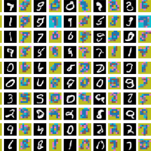
In order to train the prior, we’re going to encode every training image to obtain their discrete representation as indices in the latent codebook. This is also a good opportunity to visualize the discrete representations learned by the encoder. Here we can notice some interesting features, such as: all the black/background pixels are mapped to the same codeword, and the same for dense/white pixels (e.g., the ones at the center of a number)
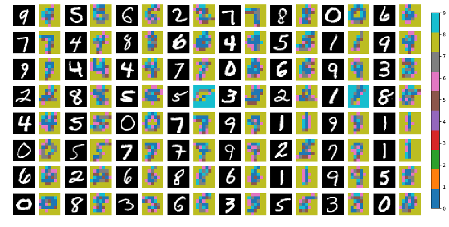
Figure 4: Visualizing categorical codes learned by the VQ-VAE encoder
Equipped with the Masked gated convolutions and the training set, we can finally build our PixelCNN architecture and train the prior. The full model simply consists in a concatenation of masked and gated convolutions, followed by two fully-connected layers to output the final prediction. Here the training objective is a multi-class classification one, as the prior should output a map of codebook indices.
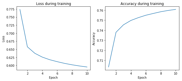
Figure 5: Training the VQ-VAE PixelCNN prior
Once again, we can check the model ability to reconstruct discrete latent codes obtained from the test set:
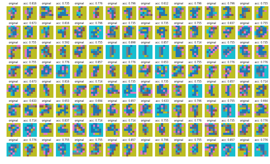
Figure 6: Training the VQ-VAE PixelCNN prior
More importantly, let’s have a look at images generated by sampling from the prior. As expected, they look much better than sampling from a uniform distribution, which means that (i) discrete codes for our image distribution lie in a specific subset of the latent space and (ii) the PixelCNN was able to properly model a prior probability distribution on that space
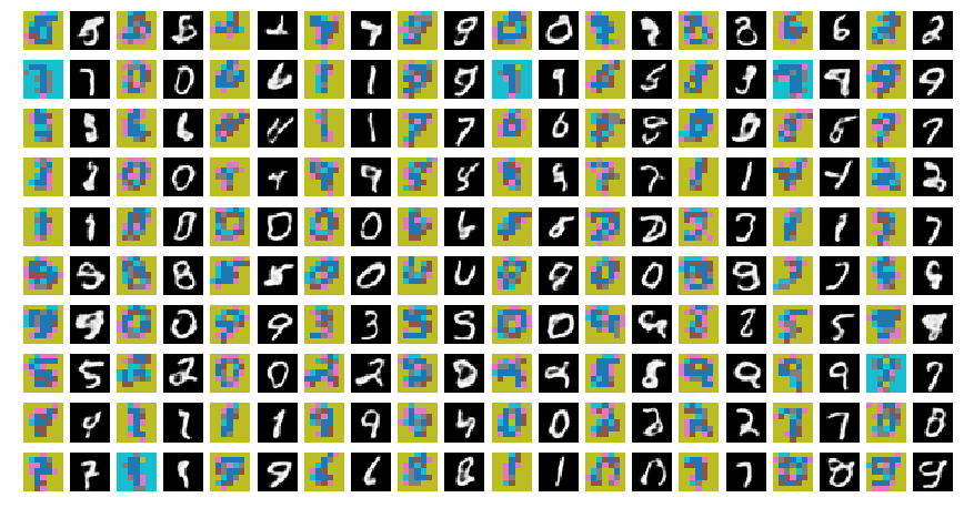
Figure 7: Generating samples from the learned PixelCNN prior
