This notebook discusses/summarizes the Deep Image Prior and a closely related follow-up work, the deep decoder, in Tensorflow 2/keras. This is an updated and simplified version of a tf v1 code repository I uploaded some time ago on github. For a more complete review of the paper, see also the reading notes.
Pros (+)
- Single-image method, no need for pre-training
- Learned prior rather than handcrafted
Cons (-)
- Over parametrized architecture (somewhat adressed by the Deep Decoder follow-up)
Deep Image Prior
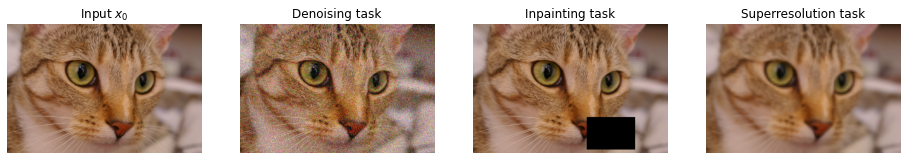
Standard inverse problem in Computer Vision (denoising, inpainting, super-resolution) can usually be phrased as a two loss terms minimization objective:
\[x^\ast = \arg\min_x E(x, x_0) + R(x)\]where $x_0$ is the input image, $E$ is a task-specific term and $R$ is a regularizer. For instance in the denoising case, $x_0$ would be the input noisy image, $E$ could be the L2-loss and a classical choice for $R$ is the total variation norm, TV.
## We'll always work with images in range [0, 1]
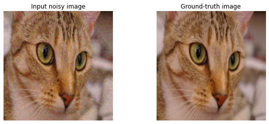
def get_noisy_img(img, sig=30):
"""Task 1: Removing white noise"""
sigma = sig / 255.
noise = np.random.normal(scale=sigma, size=img.shape)
img_noisy = np.clip(img + noise, 0, 1).astype(np.float32)
return img_noisy
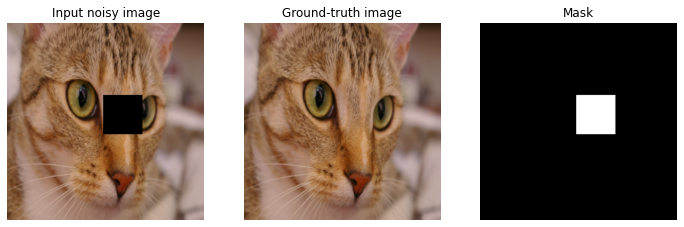
def get_inpainted_img(img, mask_size=0.25):
"""Task 2: Inpaint rectangular zero mask"""
mask = np.ones_like(img)[:, :, :1]
sx, sy = int(mask_size * img.shape[0]), int(mask_size * img.shape[1])
x = np.random.randint(0, img.shape[0] - sx)
y = np.random.randint(0, img.shape[1] - sy)
mask[x:x + sx, y:y + sy] = 0
img_noisy = img * mask
return img_noisy, mask
Neural networks as regularizers ?
Intuitively, the regularizer $R$ is task-independent and should encourage a realistic, natural-looking generated image. For instance, the total variation norm (TV) tends to favor images with uniform regions.
The main idea of the paper is to use a neural network for the regularization term, rather than an handcrafted prior, with the following high-level idea:
\[R(x) = 0\ \mbox{if}\ \exists \theta\ \mbox{s.t.}\ x = f_{\theta}(z)\\ R(x) = + \infty,\ \mbox{otherwise}\]What this regularizer says is that intuitively, our target $x^{\ast}$ is the “optimal” output (with respect to loss function $E$) that can be generated by the function $f$ from some fixed input $z$.
The workflow of the model can thus be summarized as follows
\[\mbox{Randomly initialize a neural network $f_{\theta}$ and an input $z$}\\ \mbox{Train parameters }\theta^\ast = \arg\min_{\theta} E(f_{\theta}(z),x_0) \\ \mbox{Output }x^\ast = f_{\theta^\ast}(z)\]def dip_workflow(x0,
x_true,
f,
f_input_shape,
z_std=0.1,
loss_mask=None,
num_iters=5000,
init_lr=0.01,
save_filepath=None):
"""Deep Image prior workflow
Args:
* x0: input image
* x_true: Ground-truth image, only used for metrics comparison
* f: Neural network to use as a prior
* f_input_shape: Shape (excluding batch size) of inputs to f
* loss_mask: if not None, a binary mask with the same shape as x0,
which is applied to both x and x0 before applying the loss.
Used for instance in the inpainting task.
* num_iters: Number of training iterations
* init_lr: Initial learning rate for Adam optimizer
* If True, will save the best model in the given filepath
"""
# Sample input z
shape = (1,) + f_input_shape
z = tf.constant(np.random.uniform(size=shape).astype(np.float32) * z_std, name='net_input')
# Training Loss
def loss_fn(x_true, x):
del x_true
nonlocal x0, loss_mask
if loss_mask is None:
return tf.keras.losses.MSE(x, x0)
else:
return tf.keras.losses.MSE(x * loss_mask, x0 * loss_mask)
# Output/log information
# Diff between generated image and true ground-truth
# as mean squared error and psnr (peak signal to noise ratio)
def mse_to_gt(x_true, x):
return tf.reduce_mean(tf.losses.mean_squared_error(x, x_true))
def psnr_to_gt(x_true, x, maxv=1.):
mse = tf.reduce_mean(tf.losses.mean_squared_error(x, x_true))
psnr_ = 10. * tf.math.log(maxv** 2 /mse) / tf.math.log(10.)
return psnr_
# Optimization
opt = tf.keras.optimizers.Adam(learning_rate=init_lr)
f.compile(optimizer=opt, loss=loss_fn, metrics=[mse_to_gt, psnr_to_gt])
# Saving best model
callbacks = ()
if save_filepath is not None:
callbacks = create_saving_callback(save_filepath)
# Training
history = f.fit(z,
x_true[None, ...],
epochs=num_iters,
steps_per_epoch=1,
verbose=0,
callbacks=callbacks+(TqdmCallback(verbose=1),))
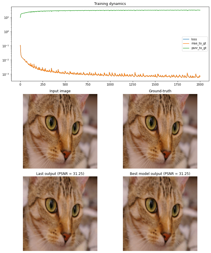
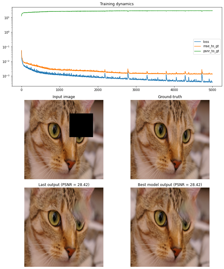
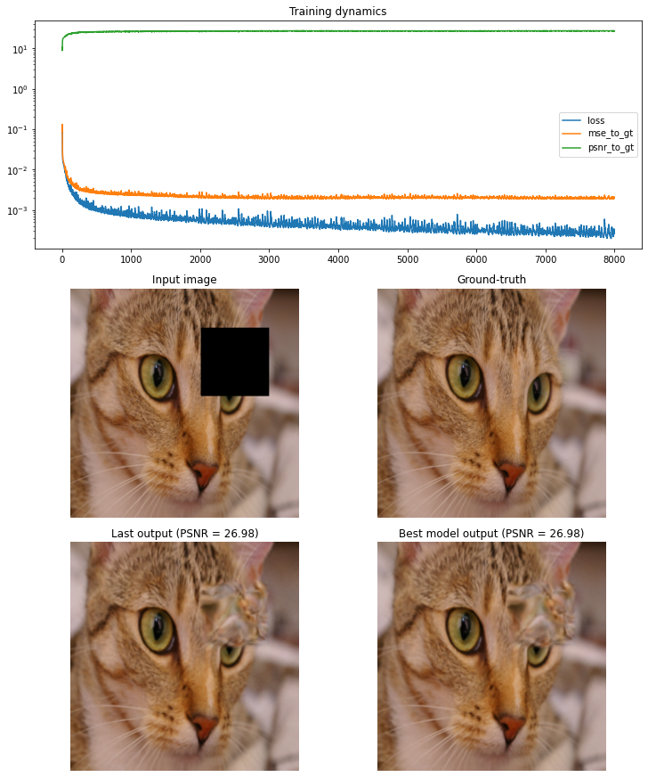
# Display results with gridspec
x = f.predict(z)[0]
fig = plt.figure(figsize=(10, 12), constrained_layout=True)
gs = fig.add_gridspec(3, 2)
axes = [fig.add_subplot(gs[0, :]),
fig.add_subplot(gs[1, 0]),
fig.add_subplot(gs[1, 1]),
fig.add_subplot(gs[2, 0]),
fig.add_subplot(gs[2, 1])]
for ax in axes[1:]:
ax.set_axis_off()
for key in history.history.keys():
axes[0].plot(range(num_iters), history.history[key], label=key)
axes[0].set_yscale('log')
axes[0].legend()
axes[0].set_title("Training dynamics")
axes[1].imshow(x0); axes[1].set_title('Input image')
axes[2].imshow(x_true); axes[2].set_title('Ground-truth')
axes[3].imshow(x); axes[3].set_title(f'Last output (PSNR = {psnr_to_gt(x_true, x):.2f})')
if save_filepath is not None and os.path.exists(save_filepath):
f.load_weights(save_filepath)
x_opt = f.predict(z)[0]
axes[4].imshow(x_opt); axes[4].set_axis_off()
axes[4].set_title(f'Best model output (PSNR = {psnr_to_gt(x_true, x):.2f})')
plt.show()
return x
Note 1: In the supplemental material, the authors also mention they sometimes use “noise-based” regularization, which consists in adding some small random noise to the input $z$ at different training iterations, with a (optionally) decaying variance.
Note 2: Another small optimization is to track the loss during training and return the image at the lowest loss point, rather than the last generated one.
Network Architecture
Deep Image Prior
The architecture used in experiments is well detailled in the supplemental material. The authors mainly experimented with “UNet” style network, i.e. encoder-decoder architecture with a bottleneck and shortcut/skip connections across the encoder and decoded between feature maps of the same spatial dimensions.
Some additional observations:
- Simpler models (less shortcut/skip paths) are usually better priors
- Leaky ReLu activations
- For upsampling, bilinear upsampling + conv 1x1 performed better than using strided transposed convolutions (see also this article on the topic). But no impact on downsampling operations.
Using keras, we can implement the proposed default architecture as follows:
def deep_image_prior(input_shape,
                     noise_reg=None,
                     layers=(128, 128, 128, 128, 128),
                     kernel_size_down=3,
                     kernel_size_up=3,
                     skip=(0, 4, 4, 4, 4)):
    def norm_and_active(x):
        x = tf.keras.layers.BatchNormalization()(x)
        x = tf.keras.layers.LeakyReLU()(x)
        return x

    model = tf.keras.models.Sequential(name="Deep Image Prior")
    inputs = tf.keras.Input(shape=input_shape)

    ## Inputs
    x = inputs
    if noise_reg is not None:
        x = GaussianNoiseWithDecay(**noise_reg)(x)

    ## Downsampling layers
    down_layers = []
    for i, (num_filters, do_skip) in enumerate(zip(layers, skip)):
        if do_skip > 0:
            down_layers.append(norm_and_active(tf.keras.layers.Conv2D(
                filters=do_skip, kernel_size=1, strides=1, name=f"conv_skip_depth_{i}")(x)))
        for j, strides in enumerate([2, 1]):
            x = norm_and_active(tf.keras.layers.Conv2D(
                num_filters, kernel_size_down, strides=strides, padding='same',
                name=f"conv_down_{j + 1}_depth_{i}")(x))

    ## Upsampling
    for i, (num_filters, do_skip) in enumerate(zip(layers[::-1], skip[::-1])):
        x = tf.keras.layers.UpSampling2D(interpolation='bilinear', name=f"upsample_depth_{i}")(x)
        if do_skip:
            x = tf.keras.layers.Concatenate(axis=-1)([x, down_layers.pop()])
        for j, kernel_size in enumerate([kernel_size_up, 1]):
            x = norm_and_active(tf.keras.layers.Conv2D(
                num_filters, kernel_size, strides=1, padding='same',
                name=f"conv_up_{j + 1}_depth_{i}")(x))

    ## Last conv
    x = tf.keras.layers.Conv2D(filters=3, kernel_size=1, strides=1, name="conv_out")(x)
    x = tf.keras.layers.Activation('sigmoid')(x)
    return tf.keras.Model(inputs=inputs, outputs=x, name="deep_image_prior")
Deep Decoder
The Deep Decoder is a follow-up work which proposes to use a much simpler, under-parametrized, architecture as a prior for these reverse tasks. In particular the architecture is non-convolutional (kernel size = 1). The deep decoder architecture combines standard blocks include linear combination of channels (convolutions ), ReLU, batch-normalization and upscaling.
As a result, it’s often easier and faster to train than the Deep Image Prior. Because of its low number of parameters, the original paper also explore using the Deep Decoder as an image compression scheme (see last section of the notebook).
def deep_decoder(input_shape,
                 noise_reg=None,
                 layers=(128, 128, 128, 128, 128),
                 kernel_size=1,
                 bn_before_act=False,
                 upsample_first=True):
    """Deep Decoder.
       Takes as inputs a 4D Tensor (batch, width, height, channels)"""
    ## Configure
    model = tf.keras.models.Sequential(name="Deep Decoder")
    inputs = tf.keras.Input(shape=input_shape)

    ## Inputs
    x = inputs
    if noise_reg is not None:
        x = GaussianNoiseWithDecay(**noise_reg)(x)


    ## Deep Decoder
    for i, num_filters in enumerate(layers):
        # Upsample (first)
        if upsample_first and i != 0:
            x = tf.keras.layers.UpSampling2D(interpolation='bilinear')(x)

        # Conv
        if kernel_size > 1:
            x = tf.keras.layers.ZeroPadding2D(int((kernel_size - 1) / 2))(x)
        x = tf.keras.layers.Conv2D(num_filters, kernel_size, strides=1, padding='valid', use_bias=False)(x)

        # Upsample (second)
        if not upsample_first and i != len(num_channels_up) - 1:
            x = tf.keras.layers.UpSampling2D(interpolation='bilinear')(x)

        # Batch Norm + activation
        if bn_before_act:
            x = tf.keras.layers.BatchNormalization(momentum=0.9, epsilon=1e-5)(x)
        x = tf.keras.layers.ReLU()(x)
        if not bn_before_act:
            x = tf.keras.layers.BatchNormalization(momentum=0.9, epsilon=1e-5)(x)

    # Final convolution
    x = tf.keras.layers.Conv2D(filters=3, kernel_size=1, strides=1, padding='valid', use_bias=False)(x)
    x = tf.keras.layers.Activation('sigmoid')(x)
    return tf.keras.Model(inputs=inputs, outputs=x, name="deep_decoder")
Experiments
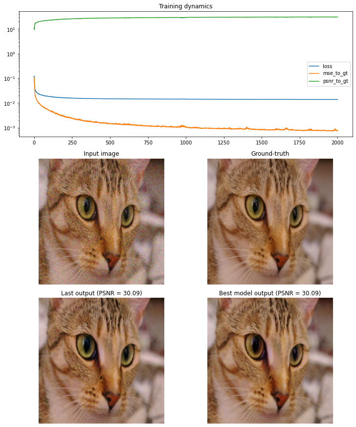
Denoising

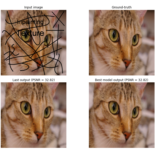
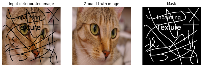
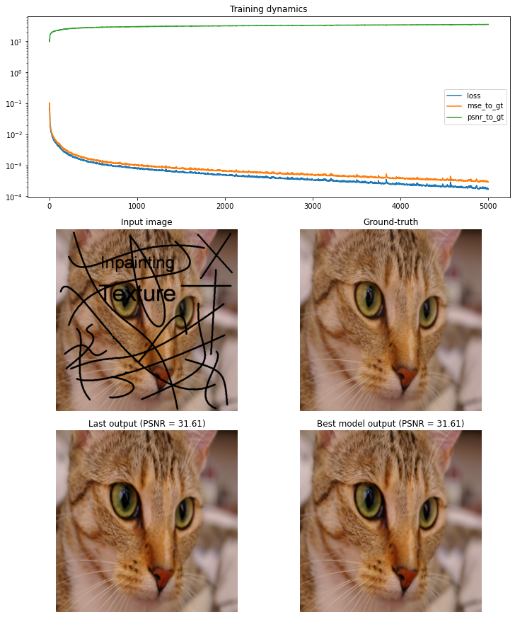
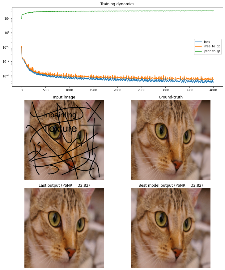
Inpainting (text)
Inpainting (hole)
Deep Decoder for Compression
One interesting property of deep decoders is that they have a low count of parameters (for instance, in the previous example, roughly 68,864 trainable parameters). This is much lower than the number of parameters in the Deep Image Prior (2M) but also much much lower than the number of pixels in the image ($512 \times 512 \times 3 = 7.8\text{M}$).
Therefore, the deep decoder can be used as a compression scheme by training the model with $x_0$ being the image to compress, and using the model itself as a compressed representation, from which the image can be generated. There is no guarantee that the model perfectly reconstructs the image, which makes it a lossy compression scheme. Finally, the compression rate is given directly by the number of parameters in the model (including the input vector $z$).
Original image: 786432 parameters
Deep Decoder (including input z): 86528 parameters
Compression rate: 9.088757396449704