This notebook discusses/summarizes the Glow generative model. For a more complete review of the paper, see also the reading notes. This code can also be found as a github repository and a kaggle notebook.
Pros (+)
- Good introduction to normalizing flows, was easy to implement from reading the paper
- Fully-reversible model: Nice interpretation in the encoder/decoder framework
- High-quality samples for a VAE based model
Cons (-)
- High memory requirements (fully-reversible means no loss of information)
- Slow training times
Glow
Glow is based on the variational auto-encoder framework with normalizing flows. A normalizing flow g is a reversible operation with an easy to compute gradient, which allows for exact computation of the likelihood, via the chain rule equation:
\[x \leftrightarrow g_1(x) \leftrightarrow \dots \leftrightarrow z\\ z = g_N \circ \dots \circ g_1(x)\\ \log p(x) = \log p(z) + \sum_{i=1}^N \log \det | \frac{d g_{i}}{d g_{i - 1}} | \ \ \ \ \ (1)\]where $x$ is the input data to model, and $z$ is the latent, as in the standard VAE framework
Note: In the Glow setup, the architecture is fully reversible, i.e., it is only composed of normalizing flow operations, which means we can compute $p(x)$ exactly. This also implies that there is no loss of information, i.e. $z$, and the intermediate variables, have as many parameters as $x$.
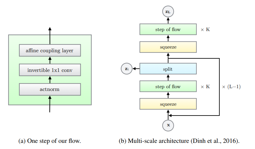
Overall architecture
Similar to Real NVP, the Glow architecture has a multi-scale structure with $L$ scales, each containing $K$ iterations of normalizing flow. Each block is separated by squeeze/split operations.
Squeeze
The goal of the squeeze operation is to trade-off spatial dimensions for channel dimensions; This preserves information, but has an impact on the field of view and computational efficiency (larger matrix multiplicatoins but fewer convolutional operations). squeeze simply splits the feature maps in 2x2xc blocks and flatten each block to shape 1x1x4c.
def squeeze(x):
    x = jnp.reshape(x, (x.shape[0],
                        x.shape[1] // 2, 2,
                        x.shape[2] // 2, 2,
                        x.shape[-1]))
    x = jnp.transpose(x, (0, 1, 3, 2, 4, 5))
    x = jnp.reshape(x, x.shape[:3] + (4 * x.shape[-1],))
    return x
And we can of course implement the reverse operation as follows:
def unsqueeze(x):
    x = jnp.reshape(x, (x.shape[0], x.shape[1], x.shape[2],
                        2, 2, x.shape[-1] // 4))
    x = jnp.transpose(x, (0, 1, 3, 2, 4, 5))
    x = jnp.reshape(x, (x.shape[0],
                        2 * x.shape[1],
                        2 * x.shape[3],
                        x.shape[5]))
    return x
Split
Intuition
The split operation essentially “retains” part of the information at each scale: The channel dimension is effectively cut in half after each scale, which makes the model a bit more lightweight computationally. This also introduces a hierarchy of latent variables.
For all scale except the last one: \(z_i, x_i = \mbox{split}(x_{i - 1})\\ x_{i} = \mbox{flow_at_scale_i}(x_i)\)
Where $z_i$ are the latent variables of the model.
def split(x):
    return jnp.split(x, 2, axis=-1)

def unsplit(x, z):
    return jnp.concatenate([z, x], axis=-1)
Learnable prior
Remember that, in order to estimate the model likelihood $\log p(x)$ in Equation (1), we need to compute the prior $p(z)$ on all the latent variables($z_1, \dots, z_L$). In the original code, the prior for each $z_i$ is assumed to be Gaussian whose mean and standard deviation $\mu_i$ and $\sigma_i$ are learned.
More specifically, after the split operation, we obtain $z_i$, the latent variable at the current scale, and $x$, the remaining output that will be propagated down the next scale. Following the original repo, we add one convolutional layer on top of $x$, to estimate the $\mu$ and $\sigma$ parameters of the prior $p(z_i) = \mathcal N(\mu, \sigma)$.
In summary, the forward pass (estimate the prior) becomes:
\[z, x = split(x_{i})\\ \mu, \sigma = \mbox{MLP}_{\mbox{prior}}(x)\\ y = \mbox{flow_at_scale_i}(x)\]and the reverse pass is
\[x = \mbox{flow_at_scale_i}^{-1}(y)\\ \mu, \sigma = \mbox{MLP}_{\mbox{prior}}(x)\\ z \sim \mathcal{N}(\mu, \sigma)\\ x = \mbox{concat}(z, x)\]The MLP is initialized with all zeros weights, which corresponds to a $\mathcal N(0, 1)$ prior. The split operation combines with the learnable prior becomes:
class ConvZeros(nn.Module):
    features: int

    @nn.compact
    def __call__(self, x, logscale_factor=3.0):
        """A simple convolutional layers initializer to all zeros"""
        x = nn.Conv(self.features, kernel_size=(3, 3),
                    strides=(1, 1), padding='same',
                    kernel_init=jax.nn.initializers.zeros,
                    bias_init=jax.nn.initializers.zeros)(x)
        return x


class Split(nn.Module):
    key: jax.random.PRNGKey = jax.random.PRNGKey(0)

    @nn.compact
    def __call__(self, x, reverse=False, z=None, eps=None, temperature=1.0):
        """Args (reverse = True):
            * z: If given, it is used instead of sampling (= deterministic mode).
                This is only used to test the reversibility of the model.
            * eps: If z is None and eps is given, then eps is assumed to be a
                sample from N(0, 1) and rescaled by the mean and variance of
                the prior. This is used during training to observe how sampling
                from fixed latents evolve.

        If both are None, the model samples z from scratch
        """
        if not reverse:
            del z, eps, temperature
            z, x = jnp.split(x, 2, axis=-1)

        # Learn the prior parameters for z
        prior = ConvZeros(x.shape[-1] * 2, name="conv_prior")(x)

        # Reverse mode: Only return the output
        if reverse:
            # sample from N(0, 1) prior (inference)
            if z is None:
                if eps is None:
                    eps = jax.random.normal(self.key, x.shape)
                eps *= temperature
                mu, logsigma = jnp.split(prior, 2, axis=-1)
                z = eps * jnp.exp(logsigma) + mu
            return jnp.concatenate([z, x], axis=-1)
        # Forward mode: Also return the prior as it is used to compute the loss
        else:
            return z, x, prior
Flow step
The normalizing flow step in Glow is composed of 3 operations:
Affine Coupling Layer: A coupling layer which splits the input data along channel dimensions, using the first half to estimate parameters of a transformation then applied to the second half (similar toRealNVP).ActNorm: Normalization layer similar to batch norm, except that the mean and standard deviation statistics are trainable parameters rather than estimated from the data (this is in particular useful here because the model sometimes has to be trained with very small batch sizes due to memory requirements)Conv 1x1: An invertible 1x1 convolution layer. This is a generalization of the channel permutation used inRealNVP
See following sections for more details on each operation.
Affine Coupling (ACL)
Forward \(x_a, x_b = \mbox{split}(x)\\ (\log \sigma, \mu) = \mbox{NN}(x_b)\\ y_a = \sigma \odot x_a + \mu\\ y = \mbox{concat}(y_a, x_b)\)
Backward \(y_a, y_b = \mbox{split}(y)\\ (\log \sigma, \mu) = \mbox{NN}(y_b)\\ x_a = (x_a - \mu) / \sigma\\ x = \mbox{concat}(x_a, y_b)\)
Log-det: $\log \det \mbox{ACL} = \sum \log (| \sigma |)$
class AffineCoupling(nn.Module):
    out_dims: int
    width: int = 512
    eps: float = 1e-8

    @nn.compact
    def __call__(self, inputs, logdet=0, reverse=False):
        # Split
        xa, xb = jnp.split(inputs, 2, axis=-1)

        # NN
        net = nn.Conv(features=self.width, kernel_size=(3, 3), strides=(1, 1),
                      padding='same', name="ACL_conv_1")(xb)
        net = nn.relu(net)
        net = nn.Conv(features=self.width, kernel_size=(1, 1), strides=(1, 1),
                      padding='same', name="ACL_conv_2")(net)
        net = nn.relu(net)
        net = ConvZeros(self.out_dims, name="ACL_conv_out")(net)
        mu, logsigma = jnp.split(net, 2, axis=-1)
        # See https://github.com/openai/glow/blob/master/model.py#L376
        # sigma = jnp.exp(logsigma)
        sigma = jax.nn.sigmoid(logsigma + 2.)

        # Merge
        if not reverse:
            ya = sigma * xa + mu
            logdet += jnp.sum(jnp.log(sigma), axis=(1, 2, 3))
        else:
            ya = (xa - mu) / (sigma + self.eps)
            logdet -= jnp.sum(jnp.log(sigma), axis=(1, 2, 3))

        y = jnp.concatenate((ya, xb), axis=-1)
        return y, logdet
Activation Norm
Forward \(y = x * \sigma + \mu\)
Backward \(x = (y - \mu) / \sigma\)
Log-det: $\log \det \mbox{ActNorm} = h \times w \times \sum \log (| \sigma |)$
Note that $\mu$ and $\sigma$ are trainable variables (contrary to batch norm) and are initialized in a data-dependant manner, such that the first batch of data used for initialization is normalized to zero-mean and unit-variance.
class ActNorm(nn.Module):
    scale: float = 1.
    eps: float = 1e-8

    @nn.compact
    def __call__(self, inputs, logdet=0, reverse=False):
        # Data dependent initialization. Will use the values of the batch
        # given during model.init
        axes = tuple(i for i in range(len(inputs.shape) - 1))
        def dd_mean_initializer(key, shape):
            """Data-dependant init for mu"""
            nonlocal inputs
            x_mean = jnp.mean(inputs, axis=axes, keepdims=True)
            return - x_mean

        def dd_stddev_initializer(key, shape):
            """Data-dependant init for sigma"""
            nonlocal inputs
            x_var = jnp.mean(inputs**2, axis=axes, keepdims=True)
            var = self.scale / (jnp.sqrt(x_var) + self.eps)
            return var

        # Forward
        shape = (1,) * len(axes) + (inputs.shape[-1],)
        mu = self.param('actnorm_mean', dd_mean_initializer, shape)
        sigma = self.param('actnorm_sigma', dd_stddev_initializer, shape)

        logsigma = jnp.log(jnp.abs(sigma))
        logdet_factor = reduce(
            operator.mul, (inputs.shape[i] for i in range(1, len(inputs.shape) - 1)), 1)
        if not reverse:
            y = sigma * (inputs + mu)
            logdet += logdet_factor * jnp.sum(logsigma)
        else:
            y = inputs / (sigma + self.eps) - mu
            logdet -= logdet_factor * jnp.sum(logsigma)

        # Logdet and return
        return y, logdet
Invertible Convolution
Forward \(y = W x\)
Backward \(x = W^{-1} y\)
Log-det: $\log \det \mbox{ActNorm} = h \times w \times \sum \log (| \det (W)|)$
In order to make the determinant computation more efficient, the authors propose to work directly with the LU-decomposition of $W$ (see original paper, section 3.2), which is initialized as a rotation matrix.
class Conv1x1(nn.Module):
    channels: int
    key: jax.random.PRNGKey = jax.random.PRNGKey(0)

    def setup(self):
        """Initialize P, L, U, s"""
        # W = PL(U + s)
        # Based on https://github.com/openai/glow/blob/master/model.py#L485
        c = self.channels
        # Sample random rotation matrix
        q, _ = jnp.linalg.qr(jax.random.normal(self.key, (c, c)), mode='complete')
        p, l, u = jax.scipy.linalg.lu(q)
        # Fixed Permutation (non-trainable)
        self.P = p
        self.P_inv = jax.scipy.linalg.inv(p)
        # Init value from LU decomposition
        L_init = l
        U_init = jnp.triu(u, k=1)
        s = jnp.diag(u)
        self.sign_s = jnp.sign(s)
        S_log_init = jnp.log(jnp.abs(s))
        self.l_mask = jnp.tril(jnp.ones((c, c)), k=-1)
        self.u_mask = jnp.transpose(self.l_mask)
        # Define trainable variables
        self.L = self.param("L", lambda k, sh: L_init, (c, c))
        self.U = self.param("U", lambda k, sh: U_init, (c, c))
        self.log_s = self.param("log_s", lambda k, sh: S_log_init, (c,))


    def __call__(self, inputs, logdet=0, reverse=False):
        c = self.channels
        assert c == inputs.shape[-1]
        # enforce constraints that L and U are triangular
        # in the LU decomposition
        L = self.L * self.l_mask + jnp.eye(c)
        U = self.U * self.u_mask + jnp.diag(self.sign_s * jnp.exp(self.log_s))
        logdet_factor = inputs.shape[1] * inputs.shape[2]

        # forward
        if not reverse:
            # lax.conv uses weird ordering: NCHW and OIHW
            W = jnp.matmul(self.P, jnp.matmul(L, U))
            y = jax.lax.conv(jnp.transpose(inputs, (0, 3, 1, 2)),
                             W[..., None, None], (1, 1), 'same')
            y = jnp.transpose(y, (0, 2, 3, 1))
            logdet += jnp.sum(self.log_s) * logdet_factor
        # inverse
        else:
            W_inv = jnp.matmul(jax.scipy.linalg.inv(U), jnp.matmul(
                jax.scipy.linalg.inv(L), self.P_inv))
            y = jax.lax.conv(jnp.transpose(inputs, (0, 3, 1, 2)),
                             W_inv[..., None, None], (1, 1), 'same')
            y = jnp.transpose(y, (0, 2, 3, 1))
            logdet -= jnp.sum(self.log_s) * logdet_factor

        return y, logdet
Final model
Normalizing flow
Combining the previous elements, we finally obtain one flow step (and its inverse pass), defined as:
class FlowStep(nn.Module):
    nn_width: int = 512
    key: jax.random.PRNGKey = jax.random.PRNGKey(0)

    @nn.compact
    def __call__(self, x, logdet=0, reverse=False):
        out_dims = x.shape[-1]
        if not reverse:
            x, logdet = ActNorm()(x, logdet=logdet, reverse=False)
            x, logdet = Conv1x1(out_dims, self.key)(x, logdet=logdet, reverse=False)
            x, logdet = AffineCoupling(out_dims, self.nn_width)(x, logdet=logdet, reverse=False)
        else:
            x, logdet = AffineCoupling(out_dims, self.nn_width)(x, logdet=logdet, reverse=True)
            x, logdet = Conv1x1(out_dims, self.key)(x, logdet=logdet, reverse=True)
            x, logdet = ActNorm()(x, logdet=logdet, reverse=True)
        return x, logdet
Glow
Once we have the flow step definition, we can finally buid the multi-scale Glow architecture. The naming of the different modules is important as it guarantees that the parameters are shared adequately between the forward and reverse pass.
class GLOW(nn.Module):
    K: int = 32                                       # Number of flow steps
    L: int = 3                                        # Number of scales
    nn_width: int = 512                               # NN width in Affine Coupling Layer
    learn_top_prior: bool = False                     # If true, learn prior N(mu, sigma) for zL
    key: jax.random.PRNGKey = jax.random.PRNGKey(0)


    def flows(self, x, logdet=0, reverse=False, name=""):
        """K subsequent flows. Called at each scale."""
        for k in range(self.K):
            it = k + 1 if not reverse else self.K - k
            x, logdet = FlowStep(self.nn_width, self.key, name=f"{name}/step_{it}")(
                x, logdet=logdet, reverse=reverse)
        return x, logdet


    @nn.compact
    def __call__(self, x, reverse=False, z=None, eps=None, sampling_temperature=1.0):
        """Args:
            * x: Input to the model
            * reverse: Whether to apply the model or its inverse
            * z (reverse = True): If given, use these as intermediate latents (deterministic)
            * eps (reverse = True, z!=None): If given, use these as Gaussian samples which are later
                rescaled by the mean and variance of the appropriate prior.
            * sampling_temperature (reverse = True, z!=None): Sampling temperature
        """

        ## Inputs
        # Forward pass: Save priors for computing loss
        # Optionally save zs (only used for sanity check of reversibility)
        priors = []
        if not reverse:
            del z, eps, sampling_temperature
            z = []
        # In reverse mode, either use the given latent z (deterministic)
        # or sample them. For the first one, uses the top prior.
        # The intermediate latents are sampled in the `Split(reverse=True)` calls
        else:
            if z is not None:
                assert len(z) == self.L
            else:
                x *= sampling_temperature
                if self.learn_top_prior:
                    # Assumes input x is a sample from N(0, 1)
                    # Note: the inputs to learn the top prior is zeros (unconditioned)
                    # or some conditioning e.g. class information.
                    # If not learnable, the model just uses the input x directly
                    # see https://github.com/openai/glow/blob/master/model.py#L109
                    prior = ConvZeros(x.shape[-1] * 2, name="prior_top")(jnp.zeros(x.shape))
                    mu, logsigma = jnp.split(prior, 2, axis=-1)
                    x = x * jnp.exp(logsigma) + mu

        ## Multi-scale model
        logdet = 0
        for l in range(self.L):
            # Forward
            if not reverse:
                x = squeeze(x)
                x, logdet = self.flows(x, logdet=logdet,
                                       reverse=False,
                                       name=f"flow_scale_{l + 1}/")
                if l < self.L - 1:
                    zl, x, prior = Split(
                        key=self.key, name=f"flow_scale_{l + 1}/")(x, reverse=False)
                else:
                    zl, prior = x, None
                    if self.learn_top_prior:
                        prior = ConvZeros(zl.shape[-1] * 2, name="prior_top")(jnp.zeros(zl.shape))
                z.append(zl)
                priors.append(prior)

            # Reverse
            else:
                if l > 0:
                    x = Split(key=self.key, name=f"flow_scale_{self.L - l}/")(
                        x, reverse=True,
                        z=z[-l - 1] if z is not None else None,
                        eps=eps[-l - 1] if eps is not None else None,
                        temperature=sampling_temperature)
                x, logdet = self.flows(x, logdet=logdet, reverse=True,
                                       name=f"flow_scale_{self.L - l}/")
                x = unsqueeze(x)

        ## Return
        return x, z, logdet, priors
Training the model
Latent Log-likelihood
Following equation (1), we now only need to compute the likelihood of the latent variables, $\log p(z)$ term; The remaining loss term is computed by accumulating the log-determinant when passing through every block of the normalizing flow.
Since each $p(z)$ is a Gaussian by definition, the corresponding likelihood is easy to estimate:
@jax.vmap
def get_logpz(z, priors):
    logpz = 0
    for zi, priori in zip(z, priors):
        if priori is None:
            mu = jnp.zeros(zi.shape)
            logsigma = jnp.zeros(zi.shape)
        else:
            mu, logsigma = jnp.split(priori, 2, axis=-1)
        logpz += jnp.sum(- logsigma - 0.5 * jnp.log(2 * jnp.pi)
                         - 0.5 * (zi - mu) ** 2 / jnp.exp(2 * logsigma))
    return logpz
Note on jax.vmap: The vmap function decorator can be used to indicate that a function should be vectorized across a given axis of its inputs (default is first axis). This is very useful to model a function that can be parallelized across a batch, e.g. a loss function like here or metrics.
Dequantization
In A note on the evaluation of generative models, the authors observe that typical generative models work with probability densities, considering images as continuous variables, even though images are typically discrete inputs in [0; 255]. A common technique to dequantize the data, is to add some small uniform noise to the input training images, which we can incorporate in the output pipeline.
In the original Glow implementation, they also introduce a num_bits parameter which allows for further controlling the quantization level of the input images (8 = standard uint8, 0 = binary images)
def map_fn(image_path, num_bits=5, size=256, training=True):
    """Read image file, quantize and map to [-0.5, 0.5] range.
    If num_bits = 8, there is no quantization effect."""
    image = tf.io.decode_jpeg(tf.io.read_file(image_path))
    # Resize input image
    image = tf.cast(image, tf.float32)
    image = tf.image.resize(image, (size, size))
    image = tf.clip_by_value(image, 0., 255.)
    # Discretize to the given number of bits
    if num_bits < 8:
        image = tf.floor(image / 2 ** (8 - num_bits))
    # Send to [-1, 1]
    num_bins = 2 ** num_bits
    image = image / num_bins - 0.5
    if training:
        image = image + tf.random.uniform(tf.shape(image), 0, 1. / num_bins)
    return image


@jax.jit
def postprocess(x, num_bits):
    """Map [-0.5, 0.5] quantized images to uint space"""
    num_bins = 2 ** num_bits
    x = jnp.floor((x + 0.5) * num_bins)
    x *= 256. / num_bins
    return jnp.clip(x, 0, 255).astype(jnp.uint8)
Note on jax.jit: The jit decorator is essentially an optimization that compiles a block of operations acting on the same device together. See also the jax doc
Inference - Sampling
Drawing a parallel to the standard VAE, we can see the encoder as a forward pass of the Glow module, and the decoder as a reverse pass (Glow$^{-1}$). However, due to the reversible nature of the network, we do not actually need the reverse pass to compute the exact training objective, $p(x)$ as it depends only on the prior $p(z)$, and from the log-determinants of the normalizing flows leading from $x$ to $z$.
In other words, we only need the encoder for the training phase. The “decoder” (i.e., reverse Glow) is used for sampling only. A sampling pass is thus:
def sample(model,
           params,
           eps=None,
           shape=None,
           sampling_temperature=1.0,
           key=jax.random.PRNGKey(0),
           postprocess_fn=None,
           save_path=None,
           display=True):
    """Sampling only requires a call to the reverse pass of the model"""
    if eps is None:
        zL = jax.random.normal(key, shape)
    else:
        zL = eps[-1]
    y, *_ = model.apply(params, zL, eps=eps, sampling_temperature=sampling_temperature, reverse=True)
    return y
Experiments
Dataset
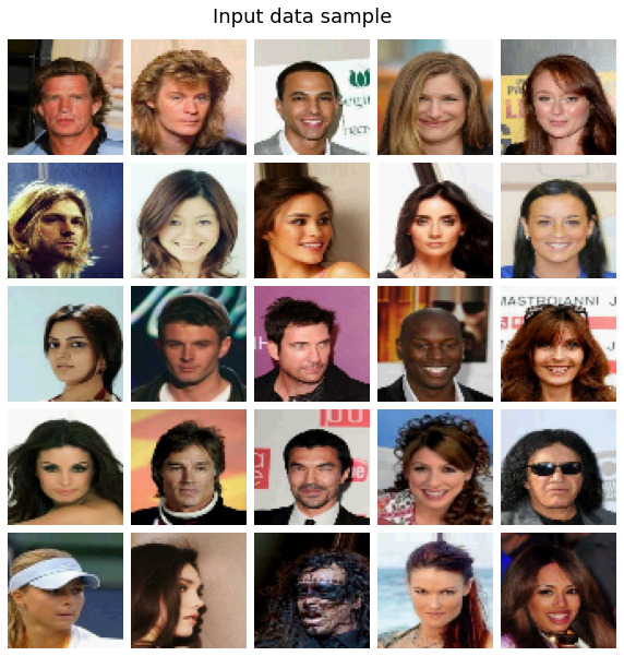
CelebA subset
- 202599 training images
- 3165 training steps per epoch
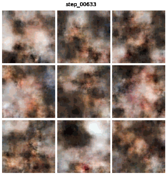
Train
Training ran for only 12 epochs due to time limits on Kaggle notebooks (roughly 40k training steps), and we also used smaller flow depth (K) than in the original paper to fit into single GPU memory.
# Data hyperparameters for 1 GPU training
config_dict = {
'image_path': "../input/celeba-dataset/img_align_celeba/img_align_celeba",
'train_split': 0.6,
'image_size': 64,
'num_channels': 3,
'num_bits': 5,
'batch_size': 64,
'K': 16,
'L': 3,
'nn_width': 512,
'learn_top_prior': True,
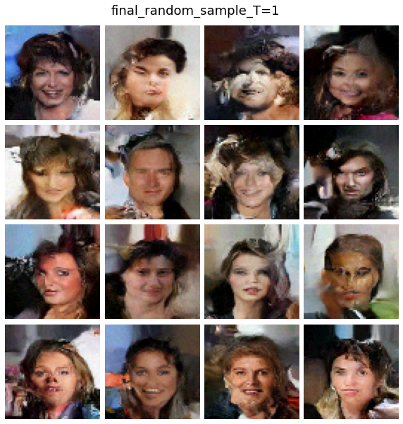
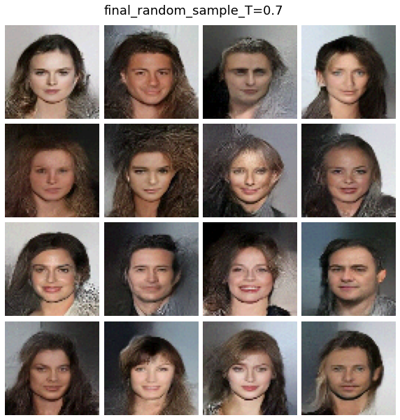
'sampling_temperature': 0.7,
'init_lr': 1e-3,
'num_epochs': 13,
'num_warmup_epochs': 1,
'num_sample_epochs': 0.2, # Fractional epochs for sampling because one epoch is quite long
'num_save_epochs': 5,
}
To visualize training, we plot the evaluation of samples drawn from the same randon imput latent variables, throughout training
Evaluation
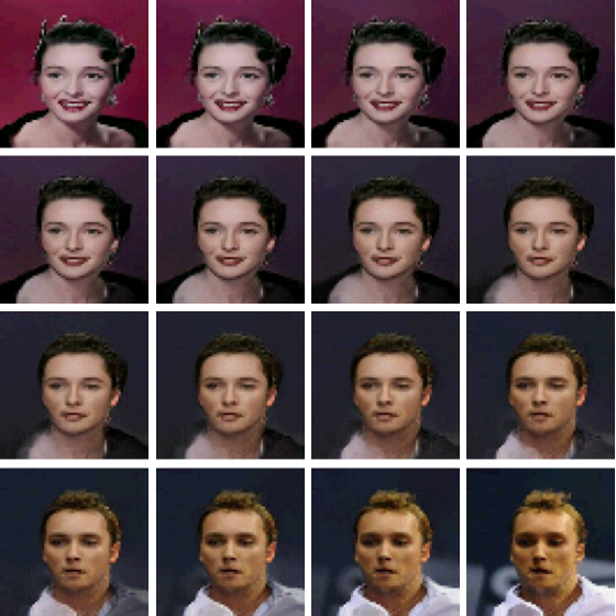
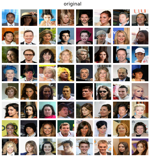
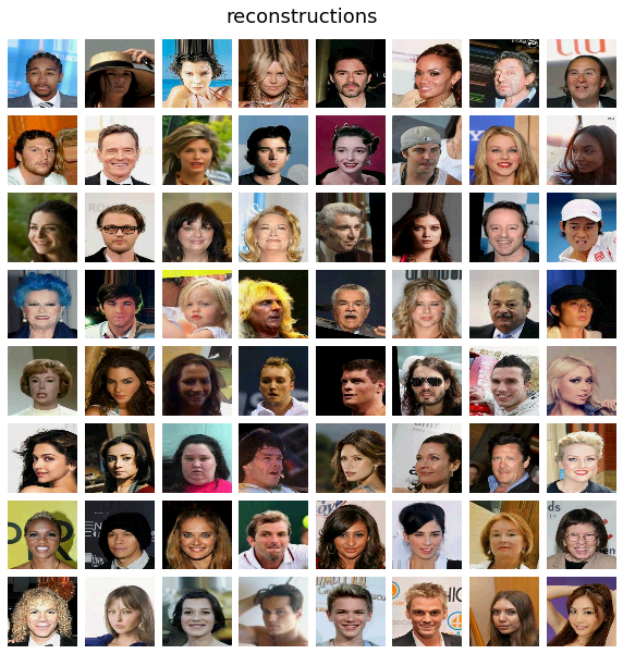
Reconstructions
As a sanity check let’s first look at image reconstructions: since the model is invertible these should always be perfect, up to small float errors, except in very bad scenarios e.g. NaN values or other numerical errors.
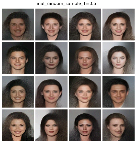
Sampling
Now let’s take some random samples from the model, starting from the learned priors, at different temperatures.
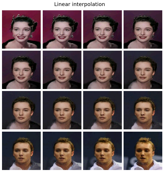
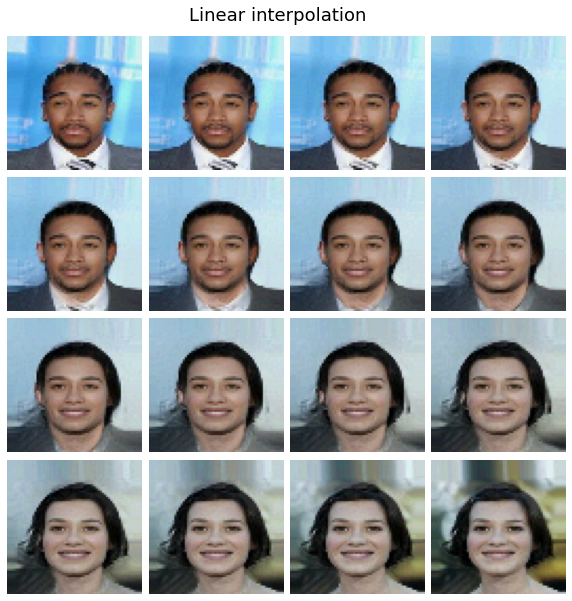
Latent space
Finally, we can look at the linear interpolation in the learned latent space: We generate embedding $z_1$ and $z_2$ by feeding two validation set images to Glow. Then we plot the decoded images for latent vectors $t + z_1 + (1 - t) z_2$ for $t \in [0, 1]$ (at all level of the latent hierarchy).
Note on conditional modeling: The model can also be extented to conditional generation (in the original code this is done by (i) learning the top prior from one-hot class embedding rather than all zeros input, and (ii) adding a small classifier on top of the output latent which should aim at predicting the correct class).
In the original paper, this allows them to do “semantic manipulation” on the Celeba dataset by building representative centroid vectors for different attributes/classes (e.g.g $z_{smiling}$ and $z_{non-smiling}$). They can use then use the vector direction $z_{smiling}$ - $z_{non-smiling}$ as a guide to browse the latent space (in that example, to make images more or less “smiling”).