
- Pros (+): Extension of
MMD-matching techniques to domain generalization: No target data available, so instead align all domains to a prior distribution - Cons (-): Potentially lacking comparison to some baselines (deep, adversarial).
Proposed model: MMD-AAE
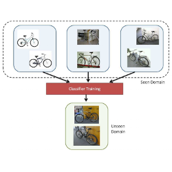
The goal of domain generalization is to find a common domain-invariant feature space underlying the source and (unseen) target spaces, under the assumption that such a space exists. To learn such space, the authors propose a variant of [1], whose goal is to minimize the variance between the different source domains distributions using Maximum Mean Discrepancy. Additionally, the source distributions are aligned with a fixed prior distribution, with the hope that this reduces the risk of overfitting to the seen domains.
Adversarial Auto-encoder
The proposed model, MMD-AAE (Maximum Mean Discrepancy Adversarial Auto-encoder) consists in an encoder \(Q: x \mapsto h\), that maps inputs to latent codes, and a decoder \(P: h \mapsto x\). These are equipped with a standard autoencoding loss to make the model learn meaningful embeddings
Based on the AAE framework [1], we also want the learned latent codes to match a certain prior distribution, \(p(h)\) (In practice, a Laplace distribution). This is done by introducing a GAN (Generative Adversarial Networks) loss term on the generated embeddings, with the prior as the true, target, distribution. Introducing \(D\), a discriminator with binary outputs, we have:
MMD Regularization
On top of the AAE objective, the authors propose to regularize the feature space using MMD, extended to the multi-domain setting. They key idea of the maximum mean discrepancy (MMD) is to compare two distributions \(\mathcal P\) and \(\mathcal Q\) using their mean statistics rather than density estimators:
A classical choice is to take \(\mathcal F\) as the space of linear functions and to leverage the kernel trick on a reproducing kernel Hilbert space to efficiently compute the difference of means
\[\begin{align} f: \ x &\mapsto \phi(x) \cdot w_{f} \tag{evaluation function}\\ \exists k,\ f(x) &= \sum_y f(y) k(x, y) = <f, k(x, \cdot) > \tag{reproducing kernel}\\ k(x, y) &= < \phi(x), \phi(y) > \end{align}\] \[\begin{align} \mathbb{E}_{x \sim \mathcal P} (f(x)) &= <f, \mathbb{E}_{x \sim \mathcal P}\ k(x, \cdot)> \overset{\Delta}{=}\ <f, \mathbf{\mu_{\mathcal P}} >\\ \text{MMD}(\mathcal P, \mathcal Q; \mathcal F) &= \sup_{f \in \mathcal F} < f, \mu_{\mathcal P} - \mu_{\mathcal Q} > = \| \mu_{\mathcal P} - \mu_{\mathcal Q} \| \end{align}\]Following [2], the authors extend this metric for multiple domains. First, we define the distributional variance to measure the dissimilarity across domains using a mean map operator, computed via the distribution over all domains, \(\bar{\mathcal P}\).
\[\begin{align} \sigma (\mathcal{P}_1, \dots, \mathcal{P}_K) = \frac{1}{K} \sum_{i=1}^K ||\mu_{\mathcal{P}_i} - \mu_{\bar{\mathcal P}} \| \end{align}\]which is 0 if and only if all the domain distributions are equal. Finally, this quantity is hard to compute but can be upper-bounded by a sum of pairwise MMDs:
In practice, the MMD is computed under a specific kernel choice and approximating the expectations by their empirical estimates.
\[\begin{align} MMD(\mathcal{P}_i, \mathcal{P}_j)^2 &= \left\| \frac{1}{n_i} \sum_t \phi(x_{i, t}) - \frac{1}{n_j} \sum_t \phi(x_{j, t}) \right \|^2\\ & = \frac{1}{n_i^2} \sum_{t, u} k(x_{i, t}, x_{i, u}) + \frac{1}{n_j^2} \sum_{t, u} k(x_{j, t}, x_{j, u}) - \frac{2}{n_i n_j} \sum_{t, u} k(x_{i, t}, x_{j, u}) \end{align}\]where \(k\) is the kernel function associated to feature map \(\phi\). Experiments are conducted with various Gaussian RBF priors.
Semi-supervised MMD-AAE
Finally, the model should learn a representation that is also adequate for the task at hand (here, classification). This is done by adding a classifier (two fully connected layers) on top of the representation minimizing a standard cross entropy loss term, \(\mathcal{L}_{\text{err}}\) between the input image label and the model output.
Experiments
Implementation
The MMD functional space uses the RBF (Gaussian) kernel. The final objective is the weighted sum of the four aforementioned loss terms (\(\mathcal{L}_{\text{AE}}, \mathcal{L}_{\text{GAN}}, \mathcal{L}_{\text{MMD}}\) and \(\mathcal{L}_{\text{err}}\)). The model is trained similarly to GANs: The discriminator and generator (auto-encoder) parameters are updated in two alternating optimization steps.
Experiments
The method is evaluated on various classification tasks (digit, object and action recognition) in settings where the domains differ by small geometric changes (e.g., change of pose). They also compare to a large range of baselines, although none of them seem to have an adversarially learned representation space (maybe [3] would have been a good additional baseline).
Additionally, ablation experiments show that the three terms \(\mathcal{L}_{\text{GAN}}\), \(\mathcal{L}_{\text{MMD}}\) and \(\mathcal{L}_{\text{err}}\) all have a positive effect on the final effect, even when taken individually.
References
- [1] Adversarial Autoencoders, Makhzani et al., ICLR Workshop, 2016
- [2] Domain Generalization via Invariant Feature Representation, Muandet et al., ICML 2013
- [3] Domain-Adversarial Training of Neural Networks, Ganin et al., JMLR 2016