- Pros (+): Interesting results, with connections to Style Transfer and Network inverson.
- Cons (-): Seems like the results might depend a lot on parameter initialization, learning rate etc.
Background
Given a random noise vector \(z\) and conditioned on an image \(x_0\), the goal of conditional image generation is to generate image \(x = f_{\theta}(z; x_0)\) (where the random nature of \(z\) provides a sampling strategy for \(x\)); for instance, the task of generating a high quality image \(x\) from its lower resolution counterpart \(x_0\).
In particular, this encompasses inverse tasks such as denoising, super-resolution and inpainting that acts at the local pixel level. Such tasks can often be phrased with an objective of the following form:
\[\begin{align} \theta^{\ast} = \arg\min E(x, x_0) + R(x) \end{align}\]where \(E\) is a cost function and \(R\) is a prior on the output space acting as a regularizer. \(R\) is often a hand-crafted prior, for instance a smoothness constraint like Total Variation [1], or, for more recent techniques, it can be implemented with adversarial training (e.g., GANs).
Deep Image Prior
In this paper, the goal is to replace \(R\) by an implicit prior captured by the neural network, relatively to input noise \(z\). In other words
\[\begin{align} R(x) &= 0\ \mbox{if}\ \exists \theta\ \mbox{s.t.}\ x = f_{\theta}(z)\\ R(x) &= + \infty,\ \mbox{otherwise} \end{align}\]Which results in the following workflow:
\[\begin{align} \theta^{\ast} = \arg\min E(f(z; x_0), x_0) \mbox{ and } x^{\ast} = f_{\theta^{\ast}}(z; x_0) \end{align}\]One could wonder if this is a good choice for a prior at all. In fact, \(f\), being instantiated as a neural network, should be powerful enough that any image \(x\) can be generated from \(z\) for a certain choice of parameters \(\theta\), which means the prior should not be constraining.
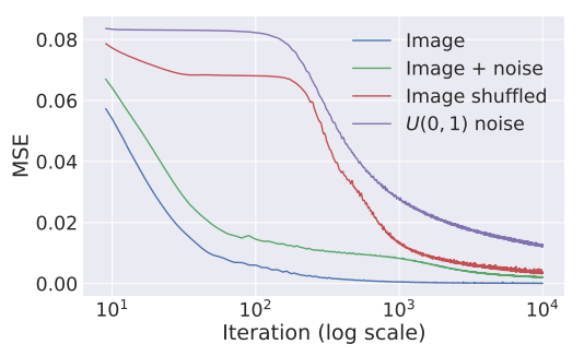
However, the structure of the network* itself effectively affects how optimization algorithms such as gradient descent will browse the output space: To quantify this effect, the authors perform a reconstruction experiment (i.e., \(E(x) = \| x - x_0 \|\)) for different choices of the input image \(x_0\) ((i)** natural image, (ii) same image with small perturbations, (iii) with large perturbations, and (iv) white noise) using a U-Net [2] inspired architecture. Experimental results show that the network descends faster to natural-looking images (case (i) and (ii)), than to random noise (case (iii) and (iv)).

Figure: Learning curves for the reconstruction task using: a natural image, the same plus i.i.d. noise, the same but randomly scrambled, and white noise.
Experiments
The experiments focus on three image analysis tasks:
- Image denoising (\(E(x, x_0) = \|x - x_0\|\)), based on the previous observation that the model converges more easily to natural-looking images than noisy ones.
- Super Resolution (\(E(x, x_0) = \| \mbox{downscale}(x) - x_0 \|\)), to upscale the resolution of input image \(x_0\)
- Image inpainting (\(E(x, x_0) = \|(x - x_0) \odot m\|\)) where the input image \(x_0\) is masked by a mask \(m\) and the goal is to recover the missing pixels.
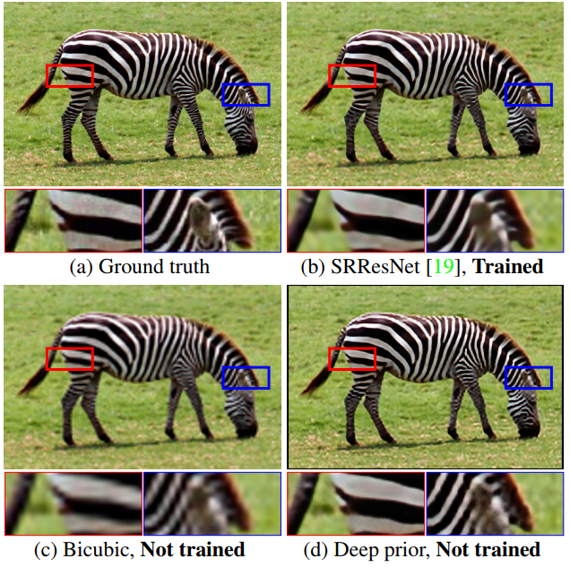
The method seems to outperform most non-trained methods, when available, (e.g. Bicubic upsampling for Super-Resolution) but is still often outperformed y learning-based ones. The inpainting results are particularly interesting, and I do not know of any other non-trained baselines for this task. Obviously performs poorly when the obscured region requires highly semantic knowledge, but it seems to perform well on more reasonable benchmarks.
Additionally, the authors test the proposed prior for diagnosing neural networks by generating natural pre-images for neural activations of deep layers. Qualitative images look better than other handcrafted priors (total variation) and are not biased to specific datasets as are trained methods.

Figure: Example comparison between the proposed Deep Image Prior and various baselines for the task of Super-Resolution.
Closely related (follow-up work)
Deep Decoder: Concise Image Representations from Untrained Non-Convolutional Networks
Heckel and Hand, [link]
This paper builds on Deep Image Prior but proposes a much simpler architecture which is under-parametrized and non-convolutional. In particular, there are fewer weight parameters than the dimensionality of the output image (in comparison, DIP was using a
U-Netbased architecture). In particular, this property implies that the weights of the network can additionally be used as a compressed representation of the image. In order to test for compression, the authors use their architecture to reconstruct image \(x\) for different compression ratios \(k\) (i.e., number of network parameters \(N\), is \(k\)-times smaller as the output dimension of the images).
The deep decoder architecture combines standard blocks include linear combination of channels (convolutions ), ReLU, batch-normalization and upscaling. Note that since here we have a special case of batch size 1, the Batch Norm operator essentially normalizes the activation channel-wise. In particular, the paper contains a nice theoretical justification for the denoising case, in which they show that the model can only fit a certain amount of noise, which explains why it would converge to more natural-looking images, although it only applies to small networks (1 layer ? possibly generalizable to multi-layer and no batch-norm)
References
- [1] An introduction to Total Variation for Image Analysis, Chambolle et al., Technical Report, 2009
- [2] U-Net: Convolutional Networks for Biomedical Image Segmentation, Ronneberger et al., MICCAI 2015

