Reading Notes
Do Deep Generative Models Know what they don't Know ?
Nalisnick et al, ICLR 2019, [link]
tags: adversarial examples - robustness - generative models - iclr - 2019
PixelCNNs and VAEs are trained to model a distribution over the input images, thus could be used to detect out-of-distribution inputs by estimating their likelihood under the data distribution. This paper provides interesting results showing that distributions learned by generative models are not robust enough yet for such purposes.
- Pros (+): Convincing experiments on multiple generative models, detailed analysis in the invertible flow case.
- Cons (-): It would be interesting to have further results for different classes of domain shifts to observe if this is rather a property of the model or of the input data. In particular results on actually detecting adversarial examples
Methodology
Three classes of generative models are considered in this paper:
- Auto-regressive models such as
PixelCNN[1] - Latent variable models such as
VAE[2] - Generative models with invertible flows [3], in particular
GLOW[4].
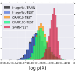
The first experiment the authors propose is to train a generative model \(G\) on input data \(\mathcal X\) and use it to evaluate the likelihood on both the training domain \(\mathcal X\) and a different domain \(\tilde{\mathcal X}\). Their first negative result is showing that a model trained on the CIFAR-10 dataset yields a higher likelihood when evaluated on the SVHN test dataset than on the CIFAR-10 test (or even train) split. Interestingly, the converse, when training on SVHN and evaluating on CIFAR, is not true. This result was consistently observed for various architectures including [1], [2] and [4], although it is of lesser effect in the PixelCNN case. Numerical results for the GLOW model are reported in Figure 1.
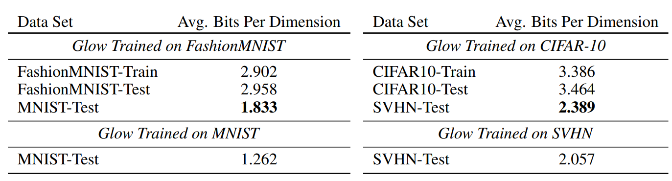
Figure 1: Testing Out-of-Distribution. Log-likelihood (expressed in bits per dimension) calculated
from GLOW on MNIST, FashionMNIST, SVHN, CIFAR-10..
Intuitively, this observation reflects the fact that both datasets contain natural images and that CIFAR-10 is strictly more diverse than SVHN in terms of semantic content, i.e., SVHN is “included” in and “easier to explain” than CIFAR. Nonetheless, these datasets vastly differ in appearance, and this result is counter-intuitive as it goes against the idea that generative models can reliably be used to detect out-of-distribution samples. Furthermore, this observation also confirms the general idea that higher likelihoods does not necessarily coincide with better generated samples [5].
Analysis in the Invertible Flow Models Case
The authors further study this phenomenon in the invertible flow models case as they provide a more rigorous analytical framework (e.g., exact likelihood estimation unlike VAEs which only provide a bound on the true likelihood).
More specifically, invertible flow models are characterized with a diffeomorphism, \(f(x; \phi)\), between input space \(\mathcal X\) and latent space \(\mathcal Z\), and a choice of prior on the latent distribution \(p(z; \psi)\). The change of variable formula links the density of \(x\) and \(z\) as follows:
\[\begin{align} \int_x p_x(x)d_x = \int_x p_z(f(x)) \left| \frac{\partial f}{\partial x} \right| dx \end{align}\]And the maximum likelihood objective under this transformation becomes
\[\begin{align} \arg\max_{\theta} \log p_x(\mathbf{x}; \theta) = \arg\max_{\phi, \psi} \sum_i \log p_z(f(x_i; \phi); \psi) + \log \left| \frac{\partial f_{\phi}}{\partial x_i} \right| \tag{1} \end{align}\]Typically, \(p_z\) is chosen to be Gaussian, and the samples are generated by applying the invert of \(f\), i.e.,\(\tilde{z} \sim p(\mathbf z),\ \tilde x = f^{-1}(\tilde z)\). For practical purposes, \(f_{\phi}\) is built such that computing the log determinant of the Jacobian terms in Equation (1) are tractable.
A first observation is that the contribution of the flow can be decomposed in a density element (left term) and a volume element (right term), resulting from the change of variables formula. Experiment results with GLOW [4] show that the higher density of SVHN under the CIFAR-trained model mostly comes from the volume element contribution.
Interestingly this esults seems quite robust: The authors also performed experiments with different types of flow formulation such as constant volume flows (where the term \(\log \left\| \frac{\partial f_{\phi}}{\partial x_i} \right\|\) is constant for all \(x\)) and with an ensemble of generative models, and still observe the same higher likelihood for SVHN.
Secondly, they try to directly analyze the difference in likelihood between two domains \(\mathcal X\) and \(\tilde{\mathcal X}\); which can be done by a second-order expansion of the log-likelihood locally around the expectation of the distribution (assuming \(\mathbb{E} (\mathcal X) \sim \mathbb{E}(\tilde{\mathcal X})\)). For the constant volume GLOW module, the final analytical formula indeed confirms that the log-likelihood of SVHN should be higher than CIFAR’s even theoretically: In some sense, SVHN is included in CIFAR (under the model distribution) and has lower variance, which explains the higher likelihood.
References
- [1] Conditional Image Generation with PixelCNN Decoders, van den Oord et al, NeurIPS 2016
- [2] Auto-Encoding Variational Bayes, Kingma and Welling, ICLR 2013
- [3] Density estimation using Real NVP, Dinh et al., ICLR 2015
- [4] Glow: Generative Flow with Invertible 1x1 Convolutions, Kingma and Dhariwal, NeurIPS 2018
- [5] A Note on the Evaluation of Generative Models, Theis et al., ICLR 2016