Reading Notes
The Variational Fair Autoencoder
Louizos et al, ICLR 2016, [link]
tags: representation learning - iclr - 2016
- Pros (+): Well justified, fast implementation trick, semi-supervised setting.
- Cons (-): requires explicit knowledge of the sensitive attribute.
Proposed
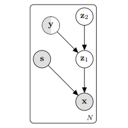
Given input data \(x\), the goal is to learn a representation of \(x\), that factorizes out nuisance or sensitive variables, \(s\), while retaining task-relevant content \(z\). Working in the VAE (Variational Autoencoder) framework, this is modeled as a generative process:
where the prior on latent \(z\) is explicitly made invariant to the variables to filter out, \(s\). Introducing decoder \(q_{\phi}: x, s \mapsto z\), this model can be trained using the standard variational lower bound objective (\(\mathcal{L}_{\text{ELBO}}\)) [1].
Semi-supervised model
In order to make the learned representations relevant to a specific task, the authors propose to incorporate label knowledge during the feature learning stage. This is particularly useful if the task target label \(y\) is correlated with the sensitive information \(s\), otherwise unsupervised learning could yield random representations in order to get rid of \(s\) only. In practice, this is done by considering two distinct independent sources of information for the latent: \(y\), the label for data point \(x\) (categorical variable in the classification scenario) and a continuous variable \(c\) that contains the remaining data variations which do not depend on \(y\) (nor \(s\)). This yields the following generative process:
\[\begin{align} y &\sim \text{Cat}(y) \mbox{ and } c \sim p(c)\\ z &\sim p_{\theta}(z | y, c)\\ x &\sim p_{\theta}(x | z, s) \end{align}\]In the fully supervised setting, when the label \(y\) is known, the ELBO can be extended to handle this two-stage latent variables scenario in a simple manner:
\[\begin{align} \mathcal{L}_{\text{ELBO}}(x, s, y) = & - \mathbb{E}_{z \sim q(\cdot | x, s)} (\log p_{\theta}(x | z, s))\tag{reconstruct}\\ & + \mathbb{E}_{z \sim q_{\phi}(\cdot | x, s)} \text{KL}(q_{\phi}(c | z, y) \| p(c))\tag{prior on c}\\ & + \mathbb{E}_{c \sim q_{\phi}(\cdot | z_1, y)} \text{KL}(q_{\phi}(z | x, s) \| p_{\theta}(z | c, y)) \tag{prior on z} \end{align}\]In the semi-supervised scenario, the label y can be missing for some of the samples. In which case, the ELBO can once again be extended to consider \(y\) as another latent variable with encoder \(q_{\phi}(y\ \vert\ z)\) and prior \(p(y)\).
MMD objective
So far, the model incorporates explicit statistical independence between the sensitive variables to protect, \(s\) and the latent information to capture from the input data, \(z\). The authors additionally propose to regularize the marginal posterior \(q_{\phi}(z\ \vert\ s)\) using the Maximum Mean Discrepancy [2]: The MMD is a distance between probability distributions that compare mean statistics, and is often combined with the kernel trick for efficient computation.
we want the latent representation to not learn any information about \(s\): This constraint can be enforced by making the distributions \(p(z\ \vert\ s = 0)\) and \(p(z\ \vert\ s = 1)\) close to one another, as measured by their MMD. This introduces a second loss term to minimize, \(\mathcal{L}_{MMD}\).
The \(MMD\) is defined as a difference of mean statistics over two distributions. Empirically, given two sample sets \(\mathbf{x^0} \sim P_0\), \(\mathbf{x^1} \sim P_1\) and a feature map operation \(\phi\), the squared distance can be written as
\[\begin{align} &\text{MMD}(P_0, P_1) =\left \| \frac{1}{|\mathbf{x^0}|} \sum_{i} \phi(\mathbf{x^0}_i) - \frac{1}{|\mathbf{x^1}|} \sum_{i} \phi(\mathbf{x^1}_i) \right\|^2\\ &= \frac{1}{|\mathbf{x^0}|^2} \left\| \sum_{i} \phi(\mathbf{x^0}_i) \right\| + \frac{1}{|\mathbf{x^1}|^2} \left\|^2 \sum_{i} \phi(\mathbf{x^1}_i) \right\|^2 - \frac{2}{|\mathbf{x^0}| |\mathbf{x^1}|} \sum_i \sum_j < \phi(\mathbf{x^0}_i), \phi(\mathbf{x^1}_j) >\\ &= \frac{1}{|\mathbf{x^0}|^2} \sum_i \sum_j k(\mathbf{x^0}_i, \mathbf{x^0}_j) + \frac{1}{|\mathbf{x^1}|^2} \sum_i \sum_j k(\mathbf{x^1}_i, \mathbf{x^1}_j) - \frac{2}{|\mathbf{x^0}| |\mathbf{x^1}|} \sum_i \sum_j k(\mathbf{x^0}_i, \mathbf{x^1}_j) \end{align}\]where the last line is the result of the kernel trick and \(k: x, y \mapsto <\phi(x), \phi(y) >\) is an arbitrary kernel function. In practice, the MMD loss term is computed over each batch: A naive implementation would require computing the full kernel matrix of \(k(x_i, x_j)\) for each pair of samples in the batch, where each scalar product requires \(K^2\) operations, where \(K\) is the dimensionality of \(x\). Instead, following [6], they use Random Kitchen Sinks [5] which is a low-rank method that allows to compute the MMD loss more efficiently.
Experiments
The authors consider three experimental scenarios to test the proposed Variational Fair Autoencoder (VFAE):
- Fairness: Here the goal is to learn a classifier while making the latent representation independent from protected information \(s\), which is a certain attribute of the data (e.g., predict “income” independently of “age”). In all the datasets considered, \(s\) is correlated with the ground-truth label \(y\), making the setting more challenging.
- Domain adaptation: Using the Amazon Reviews dataset, the task is to classify reviews as either positive or negative, coming from a supervised source domain and unsupervised target one, while being independent of the domain (i.e., book, dvd, electronics…)
- Invariant representation: Finally, the last task consists in face identity recognition while being explicitly invariant to various noise features (lighting, pose etc).
The models are evaluated on (i) their performance on the target task and (ii) their ignorance of the sensitive data. The latter is evaluated by training a classifier to prediction \(s\) from \(z\) and evaluating its performance.
On the Fairness task, the proposed method seems to be better at ignoring the sensitive information, although its trade-of between accuracy and fairness is not always the best. The main baseline is the model presented in [3], which also exploits a moment matching penalty term, although a simpler one, and does not use the VAE framework.
In the Domain Adaptation task, the authors mostly compare to the DANN [4] which proposes a simple adversarial training technique to align different domain representations. The VFAE results are on-par, or even slightly better in most scenarios.
References
- [1] Autoencoding Variational Bayes, Kingma and Welling, ICLR 2014
- [2] A Kernel Method for the Two-Sample-Problem, Gretton et al, NeurIPS 2006
- [3] Learning Fair Representations, Zemel et al, ICML 2013
- [4] Domain-Adversarial Training of Neural Networks, Ganin et al., JMLR 2016
- [5] Random Features for Large-Scale Kernel Machines, Rahimi and Recht, NeurIPS 2007
- [6] FastMMD: Ensemble of Circular Discrepancy for Efficient Two-Sample Test, Zhao and Meng, Neural Computation 2015