Reading Notes
Measuring Abstract Reasoning in Neural Networks
Barrett et al., ICML 2018, [link]
tags: visual reasoning - 2018 - icml
- Pros (+): Introduces a new dataset for abstract reasoning and different evaluation procedures, considers a large range of baselines.
- Cons (-): The Relation Network considers only pairwise interactions, might be too specific for general abstraction. Also implicit model, hard to interpret in terms of reasoning.
Dataset
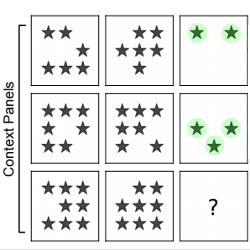
This paper introduces the Procedurally Generated Matrices (PGM) dataset. It is based on Raven’s Progressive Matrices (RPM) introduced by psychologist John Raven in 1936. Given an incomplete 3x3 matrix (missing the bottom right panel), the goal is to complete the matrix with an image picked out of 8 candidates. Typically, several candidates are plausible but the subject has to select the one with the strongest justification.
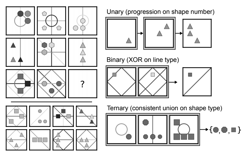
Figure: An example of PGM (left)) and depiction of relation types (right)
Construction
A PGM is defined as a set of triples \((r, o, a)\), each encoding a particular relation. For instance (progression, lines, number) means that the PGM contains a progression relation on the number of lines. In practice, the PGM dataset only contains 1 to 4 relations per PGM. The construction primitives are as follows:
- relation types (\(R\), with elements \(r\)):
progression,XOR,OR,AND,consistent union. The only relation that might require beyond binary correspondences is the consistent union. - object types (\(O\), with elements \(o\)):
shapeorlines. - attribute types (\(A\), with elements \(a\)):
size,type,colour,position,number. Each attribute takes values in a discrete set (e.g. 10 levels of gray intensity for colour).
Note that some relations are hard to define (for instance progression on shape position ?), and hence ignored. In total, 29 possible relations triples are considered.
The attributes which are not involved in any of the relations of the PGM are called the nuisance attributes. They are chosen either as a fixed value for all images in the sequence, or randomly assigned (distracting setting).
Evaluation Setting
The authors consider 8 generalization settings to evaluate on:
-
Neutral: Standard random train/test split, no constraint on the relations -
InterpolationandExtrapolation: The values of the colour and size attributes are restricted to half the possible values in the training set, and take values in the remaining half options in the test set. Note that in this setting, the test set is built such that every sequence contains one of these two attributes, i.e. generalization is required for every image. The different between inter- and extrapolation lies in the discretized space split: For interpolation, the split is uniform across the support (even-indexed values vs. odd-indexed values). In extrapolation, the values are split between lower half of the space and upper half of the space. -
Held-out: As the name indicates, this evaluation setting consists in keeping certain relations out of the training set and considering them only at test time (each of the test question contains at least one of the kept-out relations).shape-colour. Keep out any relation with \(o=\)shapeand \(a =\)colourline-type. Keep out any relation with \(o=\)lineand \(a =\)typetriples. Take out seven relation triples (chosen such that every attribute is represented exactly once.pairs of triples. Same as before but considering pairs of triples this time and only generating PGM with at least two relations: in that way, some relation interactions will have never been seen on training time.pairs of attributes. Same as before but at the attribute level
Baselines
The main contributions of the paper are to introduce the PGM dataset and evaluate several standard deep architectures on it:
-
CNN-MLP: A standard 4-layers CNN, followed by 2 fully connected layers. It takes as inputs the 8 context panels of the matrix and the 8 panel candidates concatenated on the channel axis: i.e., inputs to the model are 80x80x16 images. It outputs the labels of the correct panels (8-labels classification task).
-
ResNet. Same as before but with a
ResNetarchitecture. -
Wild resNet. This time, the candidate panels are fed separately (i.e. 8 different input, each as a 9 channel image) and a score is output for each one of them. The candidate with the highest score is chosen.
-
Context-blind ResNet. Rather a “sanity check” than a baseline, train a
ResNetthat only takes the candidate panels as inputs, no context. -
LSTM. First, each of the 16 panels is fed independently through a 4-layers CNN and the output feature maps is tagged with an index (following the sequence order). This sequence is fed through a
LSTM, whose final hidden state is passed through one linear layer for the final classification. -
RN network. The authors propose a Relation Network based on recent work [1]. Each context panel and candidate is fed through a CNN resulting in embeddings \(\{x_1 \dots x_8\}\) and \(\{c_1 \dots c_8\}\) respectively. Then for each candidate panel \(k\), the Relation Network outputs a score \(s_k\):
Additionally, they consider a semi-supervised variant where the model tries to additionally predict the relations underlying the PGM (encoded as a one-hot vector) as a meta-target. The total loss is a weighted average between the candidate classification loss term and the meta-target regression loss term.
Experiments
Overall results
The CNN-based models perform consistently badly, while LSTM provides an improvement but a small one. The Wild ResNet provides further improvement over ResNet, which shows that using a panel scoring structure is more beneficial than direct classification of the correct candidate. Finally WReN outperforms all other baselines, which could be expected as it makes use of pairwise interactions across panels. The main benefit of the method is its simplicity (Note: it could be interesting to compare again other sequential architecture on ResNet).
Different evaluation procedure
While the WReN achieves satisfying accuracy on the neutral and interpolation splits (~ 60%), as one would expect this does not hold for the more challenging settings, e.g. it significantly drops to 17% on the extrapolation setting.
More generally, it seems that the model has troubles generalizing when some attributes are never seen during the training, (e.g., extrapolation or attr.rels settings) which seems to indicate the model probably more easily picks visual properties rather than high-level abstract reasoning ones.
Detailed results
The authors also report results broken down by number of relations per matrix, relation types and attribute types(when only one relation). As one would expect, one-relation are the easiest to solve, but, interestingly, it is slightly easier to solve three-relations matrices than four-relations one, which might be because it determines a more precise answer.
As for relations, XOR and progression are the hardest to solve although the model still performs decently well on those (50%).
Closely related work
Improving Generalization for Abstract Reasoning Tasks Using Disentangled Feature Representations [4]
Steenbrugge et al., [link]
The main observation is that the previously proposed model seems to disregard high-level abstract relations (e.g. considering the poor accuracy on the extrapolation set). this paper proposes to improve the encoding step by embedding the panel in a “disentangled” space using a \(\beta\)-VAE.
There are also a few weird details in the experimental section. For instance, they claim the RN embedding has dimension 512, while it has dimension 256 (it only becomes 512 whe concatenating in \(g_{\theta}\)). Second, they use a VAE embedding has latent dimension 64 and it’s not clear why they wouldn’t use more dimensions for a fairer comparison. The encoder used is also two layers deeper .
The model yields some improvement, especially on the more challenging settings (roughly 5% at best). They however omit results in the extrapolation regime.
RAVEN: A Dataset for Relational and Analogical Visual rEasoNing [5]
Zhang et al., [link]
This paper is conceptually very similar to “ Measuring abstract reasoning in neural networks”, they also propose a new dataset for visual reasoning based on *Raven matrices** and evaluate several baselines in various testing settings.
The dataset generation process is formulated as a grammar the generated language defining instances of
PGMmatrices. Compared to thePGMdataset, they stick closer to the definition of Advanced Raven Progressive Matrices as defined in [2], and the distribution of rules seems to be quite different from thePGMdataset, for instance, rules only apply row-wise. They design 5 rule-governing attributes and 2 noise attributes. Each rule-governing attribute goes over one of 4 rules, and objects in the same component share the same set of rules, making in total 440, 000 rule annotations and an average of 6.29 rules per problem. ```
The A-SIG (Attributed Stochastic Image Grammar) contains five levels:
Scene: root nodeStructure: Defines how relations structure the scene. For instance, the Inside-Outside structure refers to a core 2x2 Inside Component (the top-left 2x2 panels) and the rest are the Outside componentsComponents: The components of the structureLayout: Defines how objects are arranged in the scene. For comparison, the PGM generation would only have one layour: 3x3 gridEntities: The individual objects that form the layout.
As for the rules, they can be split into four main categories:
Progression(-2, -1, +1, +2) -> 4 “different” rulesConstant: Which I would hardly count as a ruleArithmetic: XOR, OR, ANDDistribute Three: Equivalent to Consistent Union
\[\begin{align} x \mapsto \mbox{ReLU}(fc([x, w_n])) \end{align}\]The authors want to make use of the annotated structure of the generated matrics using a Dynamic Residual Tree (
DRT). Each Raven matrix, corresponds to a sentence sampled from the Grammar, and as such can also be represented as an annotated tree, \(T\), from scene to entities. The authors them build a residual module where single layers areReLU-activated fully-connected layers, wired according to the tree structure similar toTree-LSTM. More specifically, let us denote by \(w_n\) the label of node \(n\). Each node correspond to one layer in the residual module, as follows:
- For nodes with a single child (e.g., scene) or leaves (e.g., entities) :
\[\begin{align} x_1, \dots x_C \mapsto \mbox{ReLU}(fc(\left[\sum_c x_c , w_n\right])) \end{align}\]
- For nodes with multiple children. Denoting by \(x_1, \dots x_C\) the outputs of each child mapping :
\[\begin{align} x \mapsto DRT(x, T) + x \end{align}\]In summary, the
DRTmodule is given the input image which is fed to the nodes, starting from the leaves and going up to the root, scene, node. Finally it is made into a residual module by adding it to the input features. in other words:
For experiments, the baselines include the Wild Relation Network (
WReN) from, the CNN network from [3] that performs direct prediction, aResNet-18Network and aLSTM. They also have human performance baselines, where the test subjects are non-expert but do have some knowledge of Raven matrices. Finally, they also have an ‘oracle’ baseline (solver), which has full knowledge of the relational structure, in which case the problem is reduced to finding the correct assignment. Finally, they augment each module with aDRTresidual block, which usually they only introduce at the penultimate layer level. Except for theWReN, where theDRTis used at the end of theCNNencoder, i.e. before the relational module
Overall the experiments results are interesting, but leads to some trange conclusions:
- (i) As was shown in the
WReNpaper, theLSTMbaseline performs rather badly. What is more surprising however is that theWReNperforms significantly worse than theResNetand theCNNbaseline. In the baseWReNarchitecture, the encoder was rather small and not thin, while here it is also compared to models that useResNetas a base encoder hence it is not clear if this a failure from the relational network itself or from e.g. the encoder.- (ii) In all cases the
DRTmodule seems to provide a small boost in predictoin accuracy- (iii) Much more strange is that the authors report a significant decrease in accuracy when using auxillary training. More specifically, it does not impact the
WReNresults, but the accuracy of theResNet+DRTmodel drops from 60%s to 21%, which is extremely counter-intuitive.- (iv) Finally, they do some generalization experiments, but only on different layouts, e.g. train on images with
Centerlayout and test on3x3 grid. But again, this seems to test more the capacity of the encoder to adapt to several visual domain shifts, rather than the ability to generalize to new relations.
References
- [1] A simple neural network module for relational reasoning, Santoro et al., NeurIPS 2017
- [2] What one intelligence test measures: a theoretical account of the processing in the raven progressive matrices test, Carpenter et al
- [3] IQ of Neural Networks, Hoshen and Werman, arXiv 2017
- [4] Improving Generalization for Abstract Reasoning Tasks Using Disentangled Feature Representations, Steenbrugge et al, arXiv 2017
- [5] RAVEN: A Dataset for Relational and Analogical Visual rEasoNing, Zhang et al, CVPR 2019