Reading Notes
Deep Visual Analogy Making
Reed et al., NeurIPS 2015, [link]
tags: visual reasoning - neurips - 2015
Word2Vec embedding [1]: More specifically hey tackle the joint task of inferring a transformation from a given (source, target) pair, and applying the same relation to a new source image.
- Pros (+): Intuitive formulation; Introduces two datasets for the visual analogy task.
- Cons (-): Only consider "local" changes, i.e. geometric transformations or single attribute modifications, and rather clean images (e.g., no background).
Proposed Model
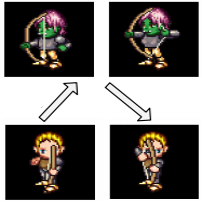
Definition: Informally, a visual analogy, denoted by “a:b :: c:d”, means that the entity a is to b what the entity c is to d. This paper focuses on the problem of generating image d after inferring the relation a:b and given a source image c.
The authors propose to use an encoder-decoder based model for generation and to model analogies as simple transformations of the latent space, for instance addition between vectors, as was the case in words embeddings such as GloVe [2] or Word2Vec [1].
Learning to generate analogies via manipulation of the embedding space
Additive objective. Let \(f\) denote the encoder that maps images to the latent space \(\mathbb{R}^K\) and \(g\) the decoder. The first, most straightforward, objective the authors consider is to model analogies as additions in the latent space:
\[\begin{align} \mathcal L_{\mbox{add}}(c, d; a, b) = \|d - g \left(f(c) + f(b) - f(a) \right)\|^2 \end{align}\]One disadvantage of this purely linear transformation is that it cannot learn complex structures such as periodic transformations: For instance, if a:b is a rotation, the the embedding for the decoded image should ideally comes back to \(f(c)\) which is not possible as we keep adding the non-zero vector \(f(b) - f(a)\). To capture more complex transformations of the latent space, the authors introduce two variants of the previous objective.
Multiplicative objective.
\[\begin{align} \mathcal L_{\mbox{mult}}(c, d; a, b) = \|d - g \left( f(c) + W \odot [f(b) - f(a)] \odot f(c) \right)\|^2 \end{align}\]where \(W \in \mathbb{R}^{K\times K\times K}\), \(K\) is the dimension of the embedding, and the three-way multiplication operator is defined as \(\forall k,\ (A \odot B \odot C)_k = \sum_{i, j} A_{ijk} B_i C_j\)
Deep objective.
\[\begin{align} \mathcal L_{\mbox{deep}}(c, d; a, b) = \|d - g \left( f(c) + \mbox{MLP}([ f(b) - f(a); f(c)]) \right)\|^2 \end{align}\]where MLP is a Multi Layer Perceptron. The \([ \cdot; \cdot]\) operator denotes concatenation. This allows for very generic transformations, but can introduce a significant number of parameters for the model to train, depending on the depth of the network.
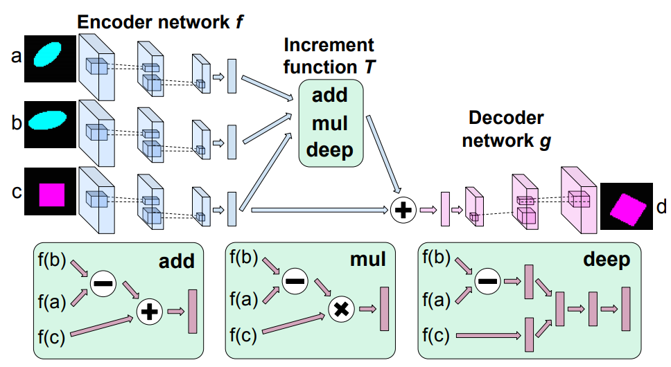
Figure: Illustration of the network structure for analogy making. The top portion shows the encoder, transformation module, and decoder. The botton portion illustrates each of the transformation variants. We share weights with all three encoder networks shown on the top left
Regularizing the latent space
While the previous losses acted at the pixel-level to match the decoded image with the target image D, the authors introduce an additional regularization loss that additionally matches the analogy at the feature level with the source analogy a:b. Formally, each objective can be written in the form \(\| d - g(f(c) + T(f(b) - f(a), f(c)))\|^2\) and the corresponding regularization loss term is defined as:
\[\begin{align} R(c, d; a, b) = \|(f(d) - f(c)) - T(f(b) - f(a), f(c))\|^2 \end{align}\]Where \(T\) is defined accordingly to match the chosen embedding, \(\mathcal L_{\mbox{add}}\), \(\mathcal L_{\mbox{mult}}\) or \(\mathcal L_{\mbox{deep}}\). For intance, \(T: (x, y) \mapsto x\) in the additive variant.
Disentangling the feature space
The authors consider another solution to the visual analogy problem, in which they aim to learn a disentangled feature space that can be freely manipulated by smoothly modifying the appropriate latent variables, rather than learning a specific operation.
In that setting, the problem is slightly different, as we require additional supervision to control the different factors of variation. It is denoted as (a, b):s :: c: given two input images a and b, and a boolean mask s on the latent space, retrieve image c which matches the features of a according to the pattern of s, and the features of b on the remaining latent variables.
Let us denote by \(S\) the number of possible axes of variations (e.g., change in illumination, elevation, rotation etc) then \(s \in \{0, 1\}^S\) is a one-hot block vector encoding the current transformation, called the switch vector. The disentangling objective is thus
\[\begin{align} \mathcal{L}_{\mbox{dis}} = |c - g(f(a) \times s + f(b) \times (1 - s))| \end{align}\]In other words the decoder tries to match c by exploiting separate and disentangled information from a and b. Contrary to the previous analogy objectives, only three images are needed, but it also requires extra supervision in the form of the switch vector s which can be hard to obtain.
Experiments
The authors consider three main experimental settings:
-
Synthetic experiments on geometric shapes. The dataset consists in 48 × 48 images scaled to [0, 1] with 4 shapes, 8 colors, 4 scales, 5 row and column positions, and 24 rotation angles. No disentangling training was performed in this setting.
-
Sprites dataset. The dataset consists of 60 × 60 color images of sprites scaled to [0, 1], with 7 attributes and 672 total unique characters. For each character, there are 5 animations each from 4 viewpoints. Each animation has between 6 and 13 frames. The data is split by characters. For the disentanglement experiments, the authors try two methods:
dist, where they only try to separate the pose from identity (i.e., only two axes of variations), anddist+cls, where they actually consider all available attributes separately. -
3D Cars. For each of the 199 car models, the authors generated 64 × 64 color renderings from 24 rotation angles each offset by 15 degrees.
The authors report results in terms of pixel prediction error. Out of the three manipulation method, \(\mathcal{L}_{\mbox deep}\) usually performs best. However qualitative samples show that \(\mathcal L_{\mbox{add}}\) and \(\mathcal L_{\mbox{mult}}\) both also perform well, although they fail for the case of rotation in the first set of experiments, which justifies the use of more complex training objectives.
Disentanglement methods usually outperforms the other baselines, especially in few-shots experiments. In particular the dist+cls method usually wins by a large margin, which shows that the additional supervision really helps in learning a structured representation. However such supervisory signal sounds hard to obtain in practice in more generic scenarios.
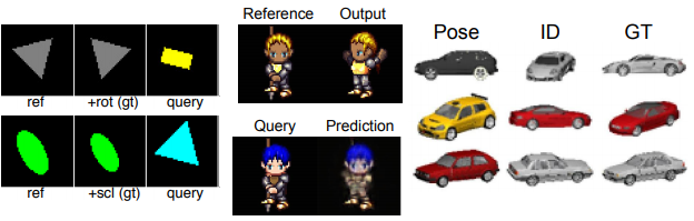
Figure 2: Examples of samples from the three visual analogy datasets considered in experiments
Closely Related
Visalogy: Answering Visual Analogy Questions [3]
Sadeghi et al., [link]
\[\begin{align} \mathcal{L}(x_{1, 2}, x_{3, 4}) = y (\| x_{1, 2} - x_{3, 4} \| -m+P) + (1 - y) \max (m_N - \| x_{1, 2} - x_{3, 4} \|, 0) \end{align}\]In this paper, the authors tackle the visual analogy problem in natural images by learning a joint embedding on relation and visual appearances using a Siamese architecture. The main idea is to learn an embedding space where the analogy transformation can be modeled by simple latent vector transformations. The model consists in a Siamese quadruple architecture, where the four heads correspond to the three context images and the candidate image for the visual analogy task respectively They do consider a restrained set of analogies, in particular those based on attributes or actions of animals or geometric view point changes. Given analogy problem \(I_1 : I_2 :: I_3 : I_4\) with label \(y\) (1 if \(I_4\) fits the analogy, 0 otherwise), the model is trained with the following objective
where \(x_{i, j}\) refers to the embedding for the image pair \(i, j\). Intuitively, the model pushes embeddings with a similar analogy close, and others apart (up to a certain margin \(m_N\)). The \(m_P\) margin is introduced as a heuristic to avoid overfittting: Embeddings are only made closer if their distance is above the margin threshold \(m_P\). The pairwise embeddings are obtained by subtracting the individual images embeddings. This implies the assumption that \(x_2 = x_1 + r\), where \(r\) is the transformation from image \(I_1\) to image \(I_2\).
The authors additionally create a visual analogy dataset. Generating the dataset is rather intuitive as long as we have an attribute-style representation of the domain. Typically, the analogies considered are transformations over properties (object, action, pose) of different categories (dog, cat, chair etc). As negative data points, they consider (i) fully random quadruples, or (ii) valid quadruples where one of \(I_3\) or \(I_4\) is swapped with a random image. The evaluation is done with image retrieval metrics. They also consider generalization scenarios: For instance removing the analogy \(white \rightarrow black\) during training, but keeping e.g. \(white \rightarrow red\) and \(green \rightarrow black\). There is a lack of details about the missing pairs to really get a full idea of the generalization ability of the model (i.e. if an analogy is missing from the training set, does that mean its reverse also is ? or does “analogy” refers to the high-level relation or is it instantiated relatively to the category too ?).
References
- [1] Distributed representations of words and phrases and their compositionality, Mikolov et al., NIPS 2013
- [2] GloVe: Global Vectors for Word Representation, Pennington et al., EMNLP 2014
- [3] Visalogy: Answering Visual Analogy Questions, Sadeghi et al., NeurIPS 2015