Reading Notes
Conditional Neural Processes
Garnelo et al, ICML 2018, [link]
tags: structured learning - graphical models - icml - 2018
- Pros (+): Novel and well justified, wide range of applications.
- Cons (-): Not clear how easy the method is to put in practice, e.g. dependency to initialization.
Proposed Model
Statistical Background
In the Conditional Neural Processes (CNP) setting, we are given \(n\) labeled points, called observations \(O = \{(x_i, y_i)\}_{i=1^n}\), and another set of \(m\) unlabeled targets \(T = \{x_i\}_{i=n + 1}^{n + m}\).We assume
that the outputs are a realization of the following process: Given \(\mathcal P\) a distribution over functions in \(X \rightarrow Y\), sample \(f \sim \mathcal P\), and set \(y_i = f(x_i)\) for all \(x_i\) in the targets set.
The goal is to learn a prediction model for the output samples while trying to obtain the same flexibility as Gaussian processes, rather than using the standard supervised learning paradigm of deep neural networks. The main inconvient of using standard Gaussian Processes is that they do not scale well (\((n + m)^3\)).
Conditional Neural Processes
CNPs give up on the theoretical guarantees of the Gaussian Process framework in exchange for more flexibility. In particular, observations are encoded in a representation of fixed dimension, independent of \(n\).
In other words, we first encode each observation and combine these embeddings via an operator \(\oplus\) to obtain a fixed representation of the observations, \(r\). Then for each new target \(x_i\) we obtain parameters \(\phi_i\) conditioned on \(r\) and \(x_i\), which determine the stochastic process to draw outputs from.
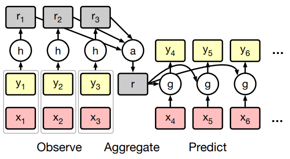
Figure: Conditional Neural Processes Architecture.
In practice, \(\oplus\) is taken to be the mean operation, i.e., \(r\) is the average of \(r_i\)s over all observations. For regression tasks, \(Q\) is a Gaussian distribution parameterized by mean and variance \(\phi = (\mu_i, \sigma_i).\) For classification tasks, \(\phi\) simply encodes a discrete distribution over classes.
Training
Given observations \(f \sim P\), \(\{(x_i, y_i = f(x_i))\}_{i=1}^n\), we sample \(N\) uniformly in \([1, \dots, n]\) and train the model to predict labels for the whole observations set, conditioned only on the subset \(\{(x_i, y_i)\}_{i=1}^N\) by minimizing the negative log likelihood:
\[\begin{align} \mathcal{L}(\theta) = - \mathbb{E}_{f \sim p} \mathbb{E}_N \left( \log Q_{\theta}(\{y_i\}_{i=1}^N |\ \{(x_i, y_i)\}_{i=1}^N, \{x_i\}_{i=1}^N) \right) \end{align}\]Note: The sampling step \(f \sim P\) is not clear, but it seems to model the stochasticity in output \(y\) given \(x\).
The mode scales with \(O(n + m)\), i.e., linear time, which is much better than the cubic rate of Gaussian Processes.
Experiments and Applications
-
1D regression: We generate a dataset that consist of functions generated from a GP with an exponential kernel. At every training step we sample a curve from the GP (\(f \sim P\)), select a subset of \(n\) points \((x_i, y_i)\) as observations, and a subset of points \((x_t, y_t)\) as target points. The output distribution on the target labels is parameterized as a Gaussian whose mean and variance are output by \(g\).
-
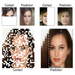
Image completion. \(f\) is a function that maps a pixel coordinate to a RGB triple. At each iteration, an image from the training set is chosen, a subset of its pixels is selected, and the aim is to predict the RGB value of the remaining pixels while conditioned on those. In particular, it is interesting to see that
CNPallows for flexible conditioning patterns, contrary to other conditional generative models which are often constrained by either the architecture (e.g.PixelCNN) or training scheme. -
Few shot classification. Consider a dataset with many classes but only few examples per class (e.g.
Omniglot). In this set of experiments, the model is trained to predict labels for samples in a select subset of classes, while being conditioned on all remaining samples in the dataset.