Reading Notes
Glow: Generative Flow with Invertible 1×1 Convolutions
D. Kingma and P. Dhariwal, NeurIPS 2018, [link]
tags: generative models - reversible networks - neurips - 2018
VAEs or GANs) and easily parallelizable training and inference (unlike the sequential generative process in auto-regressive models). This paper proposes a new, more flexible, form of invertible flow for generative models, which builds on [3].
- Pros (+): Very clear presentation, promising results both quantitative and qualitative.
- Cons (-): One of the disadvantages of the models seem to be a large number of parameters, it would be interesting to have a more detailed report on training time. Also a comparison to [5] (a variant of
PixelCNNthat allows for faster parallelized sample generation) would be nice.
Invertible flow-Based Generative Models
Given input data \(x\), invertible flow-based generative models are built as two steps processes that generate data from an intermediate latent representation \(z\):
\[\begin{align} z \sim p_{\theta}(z)\\ x = g_\theta(z) \end{align}\]where \(g_\theta\) is an invertible function, i.e. a bijection, \(g_\theta: \mathcal X \rightarrow \mathcal Z\). It acts as an encoder from the input data to the latent space. \(g\) is usually built as a sequence of smaller invertible functions \(g = g_1 \circ \dots \circ g_n\). Such a sequence is also called a normalizing flow [1]. Under this construction, the change of variables formula applied to \(x = g(z)\) gives the following equivalence between the input and latent densities:
\[\begin{align} \log p(x) &= \log p(z) + \log\ \left| \det \left( \frac{d z}{d x} \right)\right|\\ &= \log p(z) + \sum_{i=1}^n \log\ \left| \det \left( \frac{g_{\leq i}(x)}{g_{\leq i - 1}(x)} \right)\right| \end{align}\]where \(\forall i \in [1; n],\ g_{\leq i} = g_i \circ \dots g_1\) In particular, this means \(g_{\leq n}(x) = z\) and \(g_0(x) = x\). \(p_\theta(z)\) is usually chosen as a simple density such as a unit Gaussian distribution, \(p_\theta(z) = \mathcal N(z; 0, \mathbf{I})\). In order to efficiently estimate the likelihood, the functions \(g_1, \dots g_n\) are usually chosen such that the log-determinant of the Jacobian, \(\log\ \left\vert \det \left( \frac{g_{\leq i}}{g_{\leq i - 1}} \right) \right\vert\), is easily computed, for instance by choosing transformation such that the Jacobian is a triangular matrix.
Proposed Flow Construction: GLOW
Flow step
Each flow step function \(g_i\) is a sequence of three operations as follows. Given an input tensor of dimensions \(h \times w \times c\):
| Step Description | Functional Form of flow \(g_i\) | Inverse Function of the flow, \(g_i^{-1}\) | Log-determinant Expression |
|---|---|---|---|
| ActNorm \(s: [c,]\) \(b: [c,]\) |
\(y = \sigma\odot x + \mu\) | \(x = (y - \mu) / \sigma\) | \(hw\ \mbox{sum} \log(\vert\sigma\vert)\) |
| 1x1 conv \(W: [c,c]\) |
\(y = Wx\) | \(x = W^{-1}y\) | \(h w \log \vert \det (W) \vert\) |
| Affine Coupling (ACL) [2] |
\(x_a,\ x_b = \mbox{split}(x)\) \((\log \sigma, \mu) = \mbox{NN}(x_b)\) \(y_a = \sigma \odot x_a + \mu\) \(y = \mbox{concat}(y_a, x_b)\) |
\(y_a,\ y_b = \mbox{split}(y)\) \((\log \sigma, \mu) = \mbox{NN}(x_b)\) \(x_a = (y_a - \mu) / \sigma\) \(x = \mbox{concat}(x_a, y_b)\) |
\(\mbox{sum} (\log \vert\sigma\vert)\) |
-
ActNorm. The activation normalization layer is introduced as a replacement for Batch Normalization (
BN) to avoid degraded performance with small mini-batch sizes, e.g. when training with batch size 1. This layer has the same form asBN, however the bias, \(\mu\), and variance, \(\sigma\), are data-independent variables: They are initialized based on an initial mini-batch of data (data-dependent initialization), but are optimized during training with the rest of the parameters, rather than estimated from the input minibatch statistics. -
1x1 convolution. This is a simple 1x1 convolutional layer. In particular, the cost of computing the determinant of \(W\) can be reduced by writing \(W\) in its LU decomposition, although this increases the number of parameters to be learned.
-
Affine Coupling Layer. The
ACLwas introduced in [2]. The input tensor \(x\) is first split in half along the channel dimension. The second half, \(x_b\), is fed through a small neural network to get parameters \(\sigma\) and \(\mu\), and the corresponding affine transformation is applied to the first half, \(x_a\). The rescaled \(x_a\) is the actual transformed output of the layer, however \(x_b\) also has to be propagated in order to make the transformation invertible, such that \(\sigma\) and \(\mu\) can also be estimated in the reverse flow. Finally, note that the previous 1x1 convolution can be seen as a generalized permutation of the input channels, and guarantees that different channels combinations are seen during thesplitoperation.
General Pipeline
These operations are then combined in a multi-scale architecture as described in [3], which in particular relies on a squeezing operation to trade of spatial resolution for number of output channels. Given an input tensor of size \(s \times s \times c\), the squeezing operator takes blocks of size \(2 \times 2 \times c\) and flatten them to size \(1 \times 1 \times 4c\), which can easily be inverted by reshaping. The final pipeline consists in \(L\) levels that operate on different scales: each level is composed of \(K\) flow steps and a final squeezing operation.
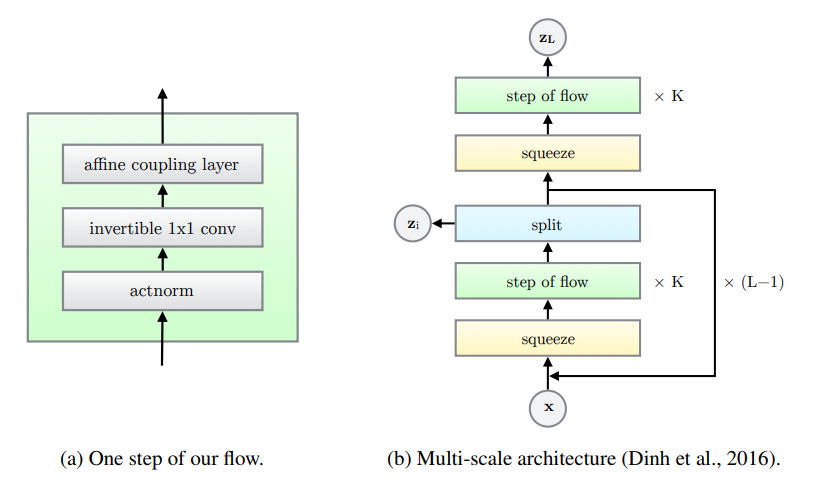
Figure: Overview of the multi-layer GLOW architecture.
In summary, the main differences with [3] are:
- Batch Normalization is replaced with Activation Normalization
- 1x1 convolutions are considered as a more generic operation to replace permutations
- Only channel-wise splitting is considered in the Affine Coupling Layer, while [3] also considered a binary spatial checkerboard pattern to split the input tensor in two.
Experiments
Implementation
In practice, the authors implement NN as a convolutional neural network of depth 3 in the ACL; which means that each flow step contains 4 convolutions in total. They also use \(K = 32\) flow steps in each level. Finally the number of levels \(L\) is 3 for small-scale experiments (32x32 images) and 6 for large scale (256x256 ImageNet images).
In particular this means that the model contains a lot of parameters (\(L \times K \times 4\) convolutions) which might be a practical disadvantage compared to other method that produce samples of similar quality, e.g. GANs. However, contrary to these models, GLOW provides exact likelihood inference.
Results
GLOW outperforms RealNVP [3] in terms of data likelihood, as evaluated on standard benchmarks (ImageNet, CIFAR-10, LSUN). In particular, the 1x1 convolutions performs better than other more specific permutations operations, and only introduces a small computational overhead.
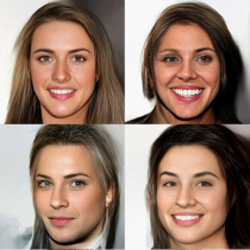
Qualitatively, the samples are of great quality and the model seems to scale well with higher resolution. However this greatly increases the memory requirements. Leveraging the model’s invertibility to avoid storing activations during the feed-forward pass such as in [4] could be used to (partially) palliate the problem.
References
- [1] Variational inference with normalizing flows, Rezende and Mohamed, ICML 2015
- [2] NICE: Non-linear Independent Components Estimation, Dinh et al., ICLR 2015
- [3] Density estimation using Real NVP, Dinh et al., ICLR 2017
- [4] The Reversible Residual Network: Backpropagation Without Storing Activations, Gomez et al., NeurIPS 2017
- [5] Parallel Multiscale Autoregressive Density Estimation, S.Reed et al, ICML 2017