Reading Notes
Learning a SAT Solver from Single-Bit Supervision
Selsam et al., ICLR 2019, [link]
tags: structured learning - logics - graphical models - iclr - 2019

SAT problems with weak supervision: In that case, a model is trained only to predict the satisfiability of a formula in conjunctive normal form. As a byproduct, if the formula is satisfiable, an actual satisfying assignment can be worked out from the network's activations in most cases.
- Pros (+): No need for extensive annotation, seems to extrapolate nicely to harder problems by increasing the number message passing iterations.
- Cons (-): Limited practical applicability since it is outperformed by classical
SATsolvers.
Model: NeuroSAT
Input
We consider boolean logic formulas in their conjunctive normal form (CNF), i.e. each input formula is represented as a conjunction (\(\land\)) of clauses, which are themselves disjunctions (\(\lor\)) of literals (positive or negative instances of variables). The goal is to learn a classifier to predict whether such a formula is satisfiable.
A first problem is how to encode the input formula in such a way that it preserves the CNF invariances (invariance to negating a literal in all clauses, invariance to permutations in \(\lor\) and \(\land\) etc.). The authors use a standard undirected graph representation where:
- \(\mathcal V\): vertices are the literals (positive and negative form of variables, denoted as \(x\) and \(\bar x\)) and the clauses occurring in the input formula
- \(\mathcal E\): Edges are added to connect (i) the literals with clauses they appear in and (ii) each literal to its negative counterpart.
The graph relations are encoded as an adjacency matrix, \(A\), with as many rows as there are literals and as many columns as there are clauses. Note that this structure does not constrain the vertices ordering, and does not make any preferential treatment between positive or negative literals. However it still has some caveats, which can be avoided by pre-processing the formula. For instance when there are disconnected components in the graph, the averaging decision rule (see next paragraph) can lead to false positives.
Message-passing model
In a high-level view, the model keeps track of an embedding for each litteral and each clause (\(L^t\) and \(C^t\)), updated via message-passing on the graph, and combined via a Multi Layer Perceptron (MLP) to output the model prediction of the formula’s satisfiability. Then the model updates are as follow:
where \(h\) designates a hidden context vector for the LSTMs. The operator \(L \mapsto \bar{L}\) returns \(\overline{L}\), the embedding matrix \(L\) where the row of each litteral is swapped with the one corresponding to the literal’s negation. In other words, in (1) each clause embedding is updated based on the litteral that composes it, while in (2) each litteral embedding is updated based on the clauses it appears in and its negated counterpart.
After \(T\) iterations of this message-passing scheme, the model computes a logit for the satisfiability classification problem, which is trained via sigmoid cross-entropy:
\[\begin{align} L^t_{\mbox{vote}} &= \texttt{MLP}_{\texttt{vote}}(L^t)\\ y^t &= \mbox{mean}(L^t_{\mbox{vote}}) \end{align}\]Building the training set
The training set is built such that for any satisfiable training formula \(S\), it also includes an unsatisfiable counterpart \(S'\) which differs from \(S\) only by negating one litteral in one clause. These carefully curated samples should constrain the model to pick up substantial characteristics of the formula. In practice, the model is trained on formulas containing up to 40 variables, and on average 200 clauses. At this size, the SAT problem can still be solved by state-of-the-art solvers (yielding the supervision required to solve the model) but are large enough they prove challenging for Machine Learning models.
Inferring the SAT assignment
When a formula is satisfiable, one often also wants to know a valuation (variable assignment) that satisfies it. Recall that \(L^t_{\mbox{vote}}\) encodes a “vote” for every literal and its negative counterpart. Qualitative experiments show that those scores cannot be directly used for inferring the variable assignment, however they do induce a nice clustering of the variables (once the message passing has converged). Hence an assignment can be found as follows:
- (1) Reshape \(L^T_{\mbox{vote}}\) to size \((n, 2)\) where \(n\) is the number of literals.
- (2) Cluster the litterals into two clusters with centers \(\Delta_1\) and \(\Delta_2\) using the following criterion: \begin{align} |x_i - \Delta_1|^2 + |\overline{x_i} - \Delta_2|^2 \leq |x_i - \Delta_2|^2 + |\overline{x_i} - \Delta_1|^2 \end{align}
- (3) Try the two resulting assignments (set \(\Delta_1\) to true and \(\Delta_2\) to false, or vice-versa) and choose the one that yields satisfiability if any.
In practice, this method retrieves a satistifiability assignment for over 70% of the satisfiable test formulas.
Experiments
In practice, the NeuroSAT model is trained with embeddings of dimension 128 and 26 message passing iterations. The MLP architectures are very standard: 3 layers followed by ReLU activations. The final model obtains 85% accuracy in predicting a formula’s satisfiability on the test set.
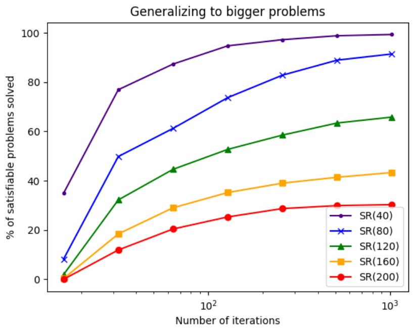
It also can generalize to larger problems, although it requires to increase the number of message passing iterations. However the classification performance significantly decreases (e.g. 25% for 200 variables) and the number of iterations linearly scales with the number of variables (at least in the paper experiments).


Figure: (left) Success rate of a NeuroSAT model trained on 40 variables for test set involving formulas with up to 200 variables, as a function of the number of message-passing iterations. (right) The sequence of literal votes across message-passing iterations on a satisfiable formula. The vote matrix is reshaped such that each row contains the votes for a literal and its negated counterpart. For several iterations, most literals vote unsat with low confidence (light blue). After a few iterations, there is a phase transition and all literals vote sat with very high confidence (dark red), until convergence.
Interestingly, the model generalizes well to other classes of problems that were reduced to SAT (using SAT’s NP-completitude), although they have different structure than the random formulas generated for training, which seems to show that the model does learn some general characteristics of boolean formulas.
To summarize, the model takes advantage of the structure of Boolean formulas, and is able to predict whether an input formula is satisfiable or not with high accuracy. Moreover, even though trained only with this weak supervisory signal, it can work out a valid assignment most of the time. However it is still subpar compared to standard SAT solvers, which makes its applicability limited.